Hello Folks! Welcome back. In this post, I will discuss the theory behind linear regression models, one of the wildly used machine learning models to predict continuous variables (fancy terms to say that we are predicting a number, also referred to as numerical target or label). The model is quite simple to understand yet powerful. We use it when model interpretability (when we want to know which dependent variables, aka features, are the most predictive) is required, like in the consumer lending or medical fields where transparency is at its core. In the next post, we will dive deeper into the coding part of a Linear Regression.

This post is the first (certainly not my last) post I have used ChatGPT to help me. ChatGPT did not write this post, of course. I used it in the ideation process, brainstorming, and breaking down some of the topics that I needed help understanding (or thought I understood) to come up with more straightforward explanations that everyone without an extensive academic background could easily understand. ChatGPT is a game changer. Sadly, most people in 2023 have yet to realize that. The world of tomorrow belongs to people who will effectively enhance their abilities and knowledge using AI systems. AI is here to stay; we must embrace innovation because no one can stop it or should.

Going back to linear regression, I have briefly discussed linear regression in this post, where we were debunking the myth “Does money buys happiness?” (spoiler alert! we found out that it does) using a simple linear regression model. In this post, we will dive deeper and discuss the main ideas about linear regression like sum square root (SSR), mean square error (MSE), R-square, and p-value, and finally, touch a little bit on derivate and gradient descent in regards to linear regression (model optimization). We will demonstrate all these with code in Python in the next blog post. This one is just the theoretical part of it. Let’s get started!

Definition

Linear regression is part of the linear models family (which assumes a linear relationship between the dependent and independent variables). This family also comprises Logistic Regression (I will have a post on this model very soon), Poisson Regression, Probit Regression, Linear Discriminant Analysis (LDA), and Cox Proportional Hazards Regression. The goal of linear regression is to fit a line (using the best parameter of a straight line, the slope “m”) to the data that minimizes the loss function or cost function (the difference between the predicted output of a machine learning model and the actual output). The loss function helps us measure how well the model performs given a dataset. The lower the loss function is, the better the model performs. The loss or cost function is also called error or residual. For the rest of this post, I will use error to refer to the loss function.

Illustration

Let’s use a simple example to illustrate and understand linear regression pragmatically; let’s say you are your country’s president’s economic advisor. Rumors say that the country is on the brink of an imminent recession from what the economists say, and the R word is on everyone’s lips in the media. Surprisingly, the unemployment number looks very low. Now the president asks you: “what is the correlation (mutual relationship) between the unemployment rate and consumer spending rate since we know that consumer spending constitutes 70% of our GDP?”. He remembers correctly from the economic class he took in university that as the employment rate increases, we should also expect consumer spending to increase. As more people are employed and have more money to spend, we should not fear a recession. So he is confused and needs some clarification of what is going on.

As a data nerd, you know that the best way to answer his question is with numbers, and you know what the saying is, right? The numbers don’t lie, so you gather all the unemployment and consumer spending data and start to investigate.

For illustration purposes, you decide to sample the data of 5 random cities in your country.

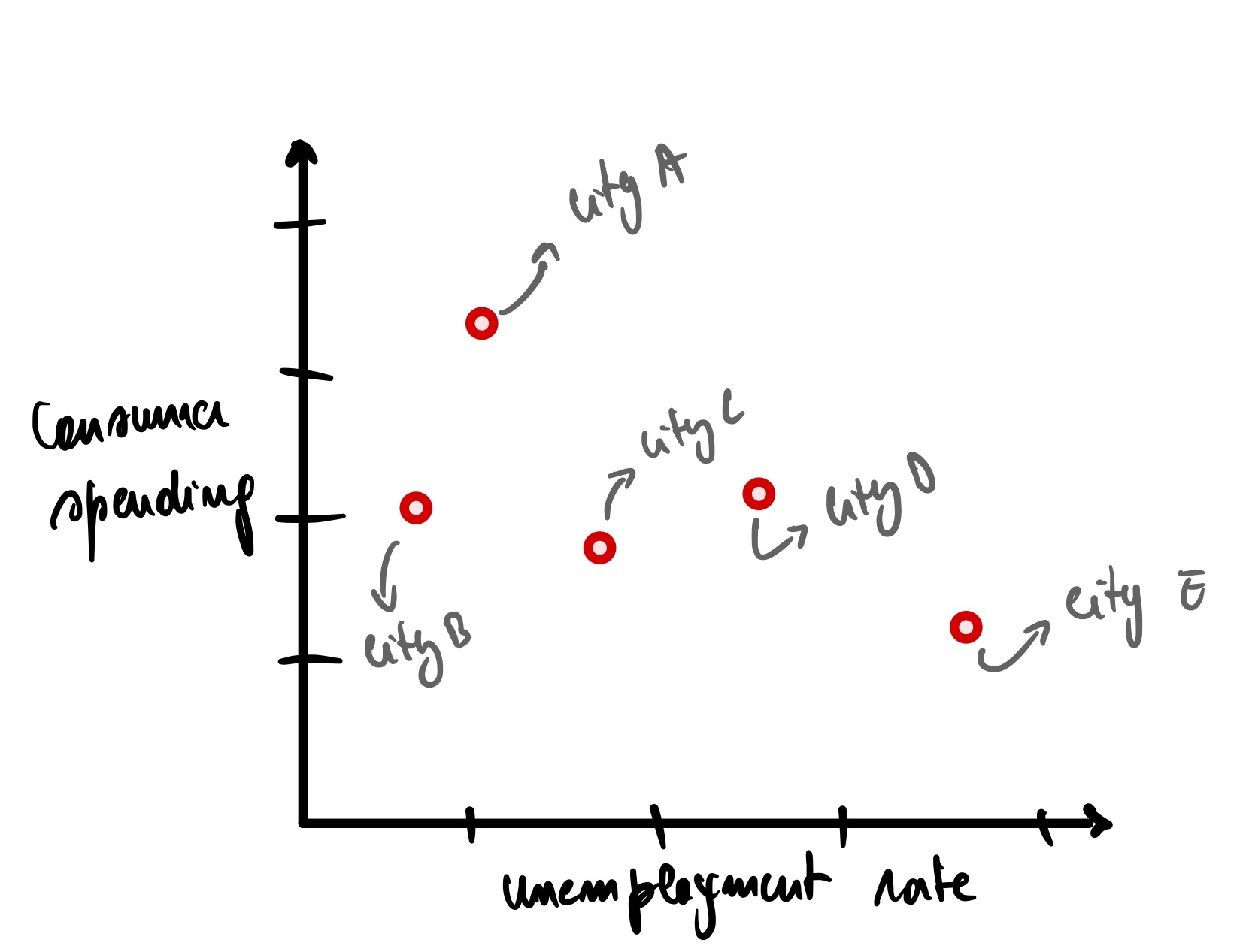
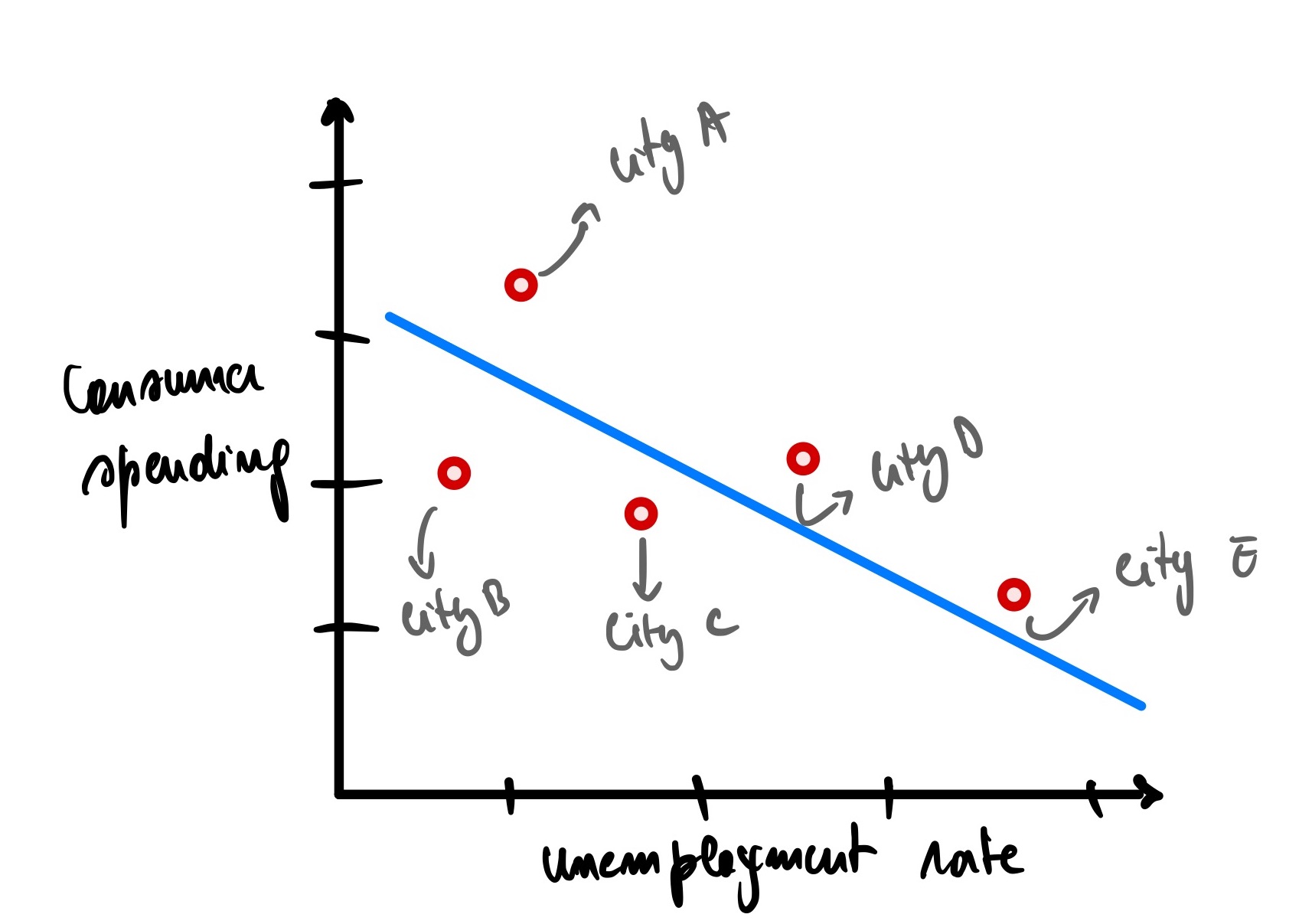
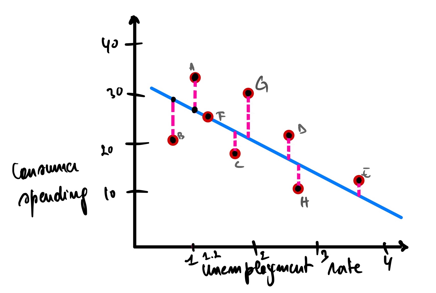
We can see that there is a downward trend here. The more the unemployment rate rises, the less consumer spending in the economy. It makes sense; as people lose their job, they tend to tighten their belts (financially speaking). We can draw a blue line of best fit to visualize this.

We can use this line to predict the consumer spending of city F given its unemployment rate of 1.2

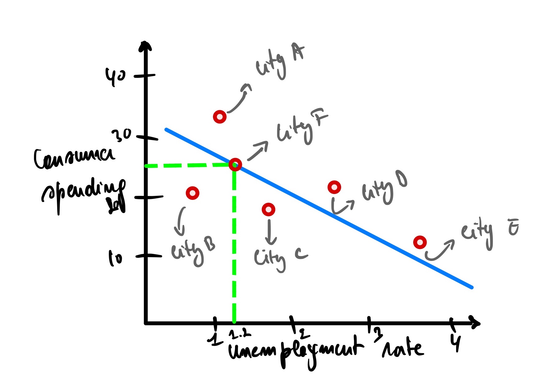
Using the graph, given an unemployment rate of city F = 1.2, the predicted consumer spending is 25.

Sum Squared Error (SSE)

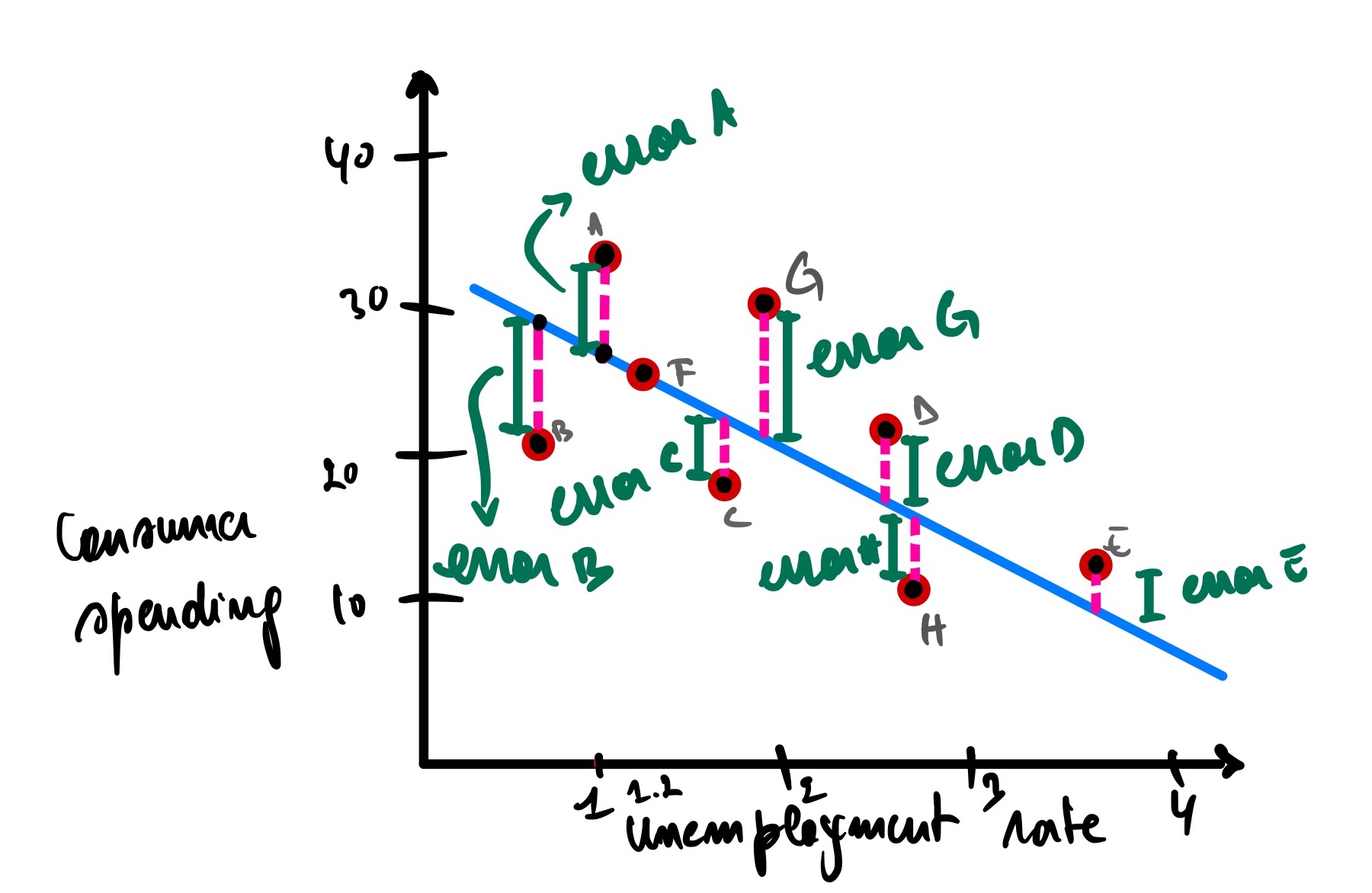
However, our model is not perfect (and it should not be because otherwise, it might be overfitting the data, meaning we won’t be able to predict untrained data). It has errors (also called residual, as discussed earlier), meaning it has actual and predicted data.

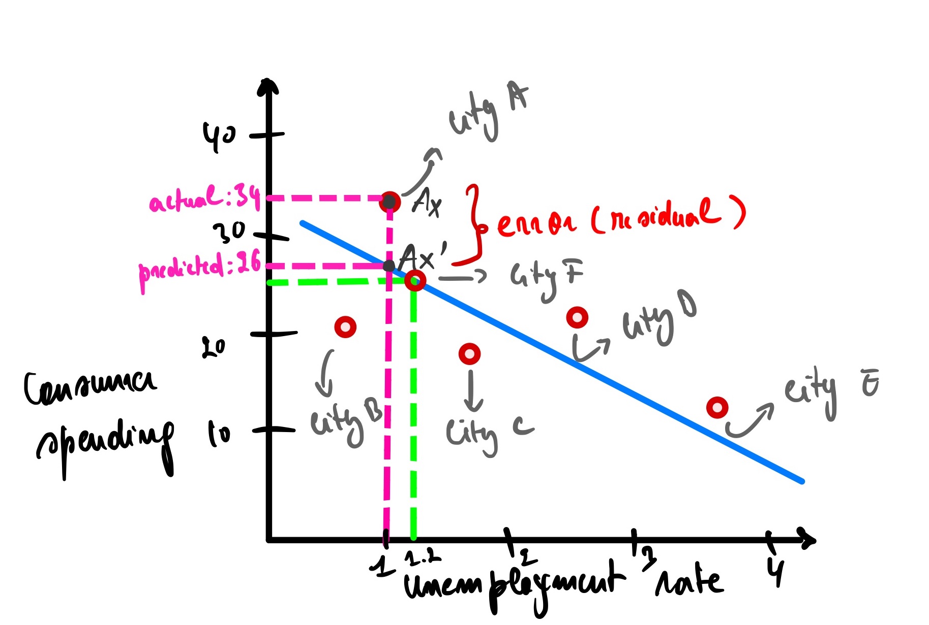
Analyzing the graph above, city A has an unemployment rate of 1, and the actual consumer spending for this city is 34 (let’s call it Ax), but our model predicts that the consumer spending is 26 (Ax’). There is an error of Ax(actual consumer spending) - Ax’(predicted consumer spending) = 34 - 26 = 8.

Same as city B, but this time the error is a negative because it is under the blue line.

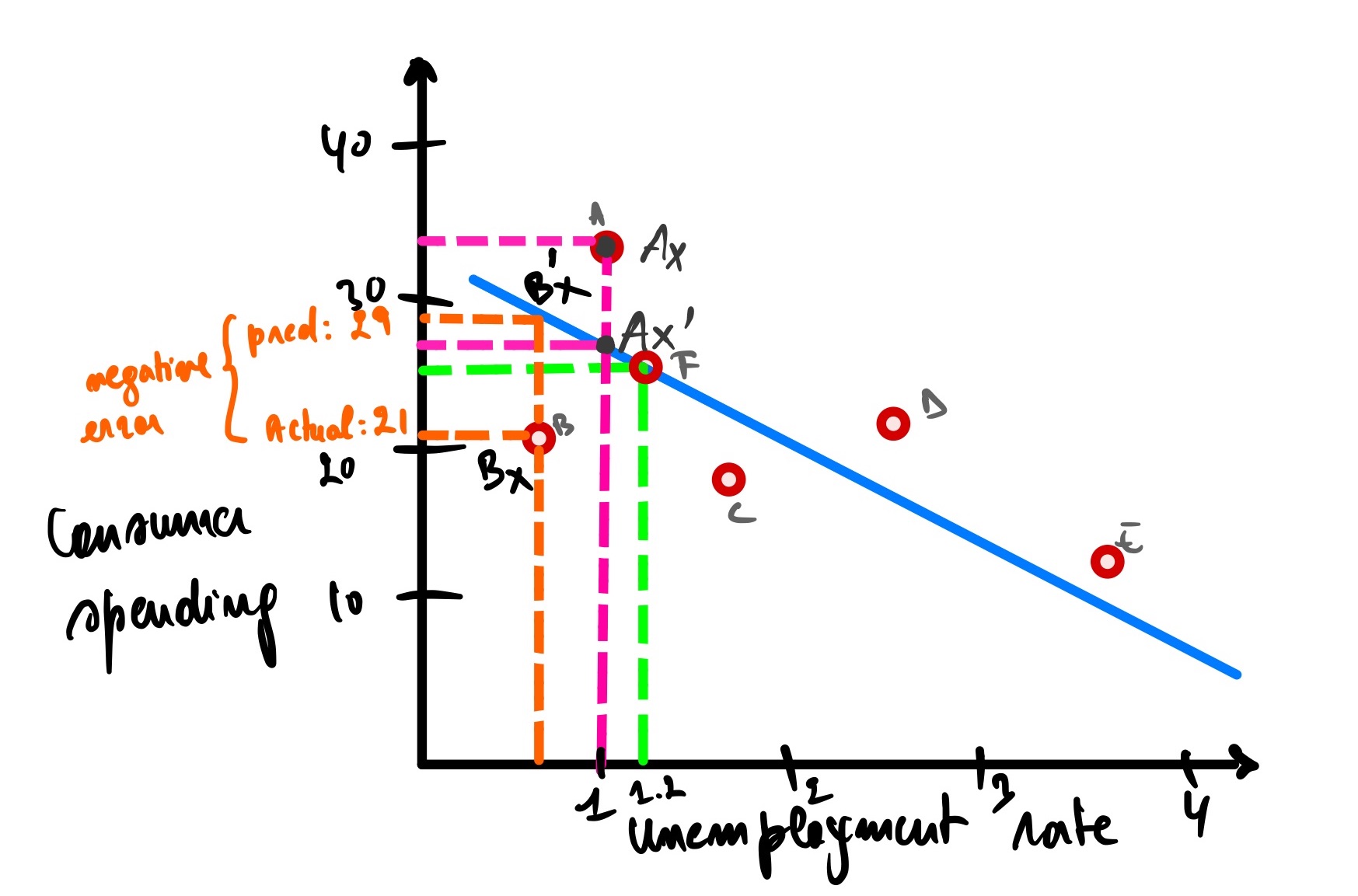
The error for city B is equal to Bx - Bx’ = 21 - 29 = -8

So now, to get the total error of all the cities, we summate all errors for each city.

(Ax - Ax’) + (Bx - Bx’) + (Cx - Cx’) + (Dx - Dx’) + (Ex - Ex’) + (Fx - Fx’)

The problem with this expression is that some errors are negative values, which will cancel out the positive ones. One way to overcome this is to use the absolute value, but a better way is to square the difference between the actual and predicted values since we will be using square root functions.

(Ax - Ax’)² + (Bx - Bx’)² + (Cx - Cx’)² + (Dx - Dx’)² + (Ex - Ex’)² + (Fx - Fx’)²

We can abbreviate it like this

∑(yᵢ - ȳ)²

Where:

• yᵢ represents the actual consumer spending of the i-th city
• ȳ represents the predicted consumer spending of the i-th city
• ∑ represents the summation

The smaller the result, the smaller the error the linear regression makes, and the better our linear regression fits our data. Our objective is to minimize it as much as we can.

The result is called Sum Squared Error (SSE), also called Sum Squared Residual (SSR).

SSE = SSR = ∑(yᵢ - ȳ)²

So the SSE in this case, is equal to

(Ax - Ax’)² + (Bx - Bx’)² + (Cx - Cx’)² + (Dx - Dx’)² + (Ex - Ex’)² + (Fx - Fx’)² =

(34 - 26)² + (21 - 29)² + (18 - 24)² + (23 - 17)² + (13 - 10)² + (26 - 26)² =

16 + 16 + 36 + 36 + 9 + 0 = 153

With the SSE of this linear regression = 153, finding another linear regression with an SSE < 153 means that this linear regression is worse than the first one. Another linear regression > 153 indicates that this last one is better than the first one.

SSE is one of the metrics used to assess a linear regression, but it has one significant drawback: Adding more data (cities in our case) will keep increasing our SSE. Let’s say; for example, we are adding cities G and H

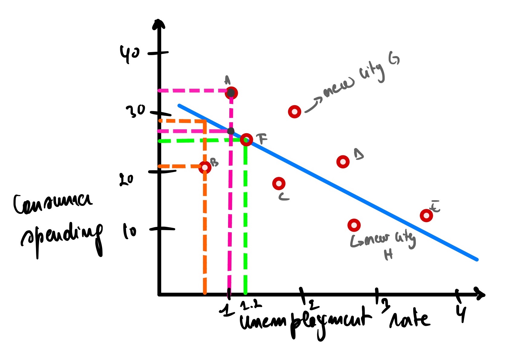
Now to calculate the new SSE with the new cities included = 153 + (Gx - Gx’)² + (Hx - Hx’)² = 153 + (31 - 23)² + (10 - 15)² = 153 + 64 + 25 = 242

Now we have a new SSE of 242. Would you conclude that this new linear regression with 7 cities is worse than that with 5? Of course not, so having a higher SSE does not always implies the worst model.

This is the main disadvantage of using SSE.

So how do we overcome this issue? Enter Mean Square Error(MSE)

Mean Squared Error (MSE)

The mean squared error is very similar to the sum square error; the only difference is that it is insensible to the number of data we have. If we add more cities, it would not drastically change the MSE.

How is the MSE different from the SSE? We divide the SSE with the number of data (n), and that’s it!

The formula of MSE is ∑(yᵢ - ȳ)²/n

Let’s see this in practice.

So to find the MSE of the six cities(A, B, C, D, E, F), we take the SSE of 153 and then divide it by 6 = 25.5

So now let’s find the MSE of the 8 cites(A, B,C, D,E, F,G, H); we take the SSE of 242 then divide it by 8 = 30.25 which is not far off to 25.5

MSE is a better metric to use than SSE, but this metric could also be better; let’s see this in an example.

Let’s change the scale of how we are expressing the dependent variable(consumer spending), so instead of expressing it in units of 10s, let’s define it in units of 10,000s

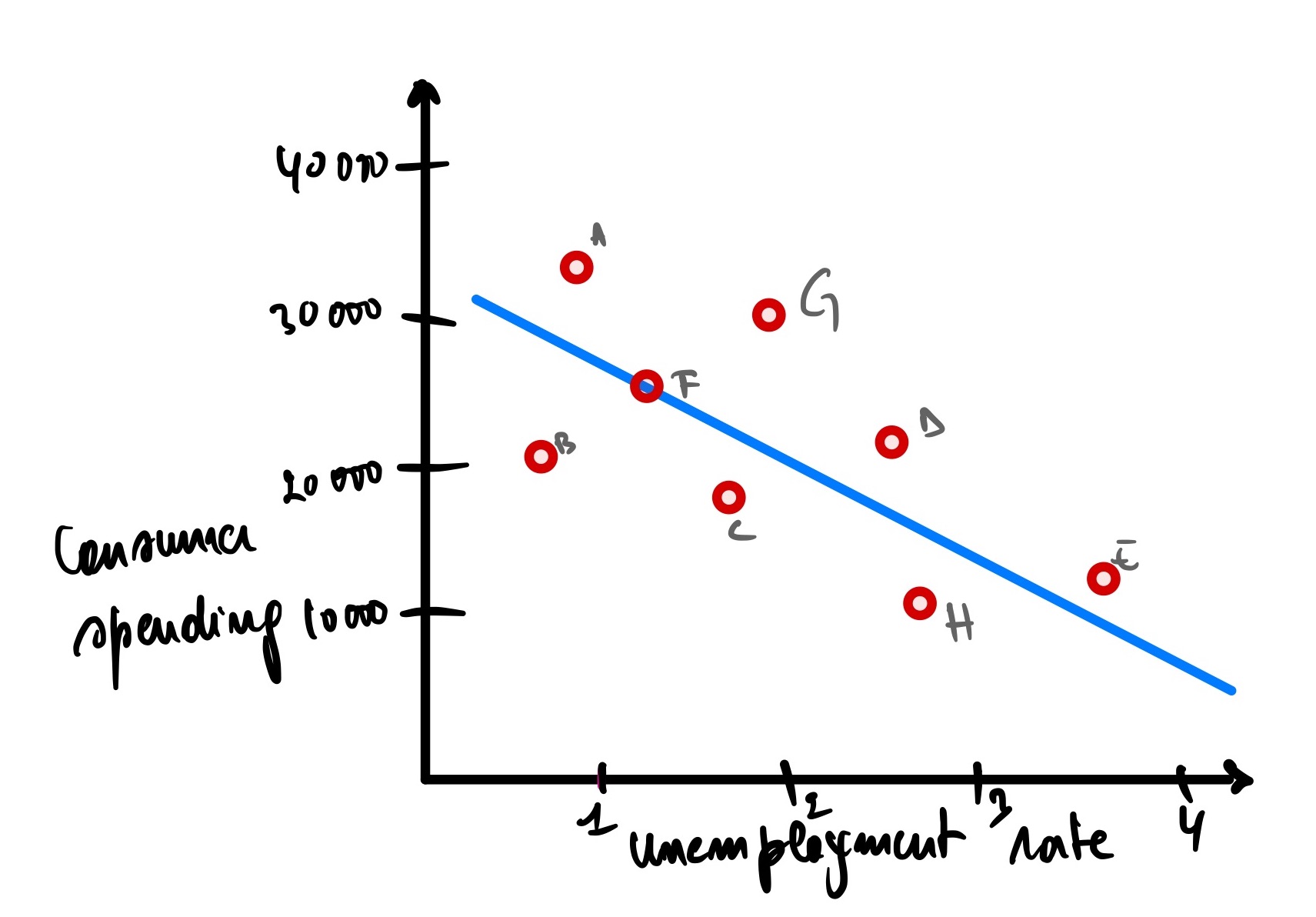
Now let’s calculate the MSE = 242 000/8 = 30250, which is way larger than the 30.25 we had before.

This is the main disadvantage of using MSE.

So how can we keep almost the same MSE even though the target scale has changed? R-squared (R²) is the answer.

R-squared

R-squared overcomes the drawbacks of SSE and MSE, which are the number of data points and the scale of the predicted variable. In other words, R-squared does not depend on the data’s size or scale. R-squared is the preferred metric for linear regression (this is not written in stone, it also depends on the type of problem you are solving), and we can calculate it from either MSE or SSE, whichever is at hand.

Let’s understand how R² works behind the scene.

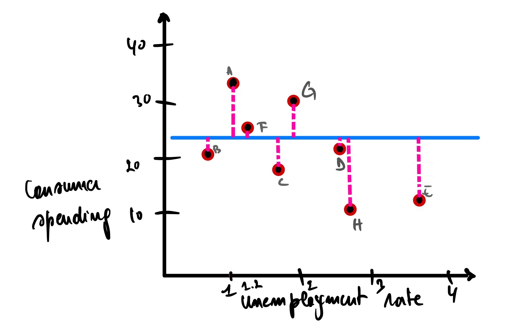
First, we calculate the data’s SSE (or MSE) around the mean.

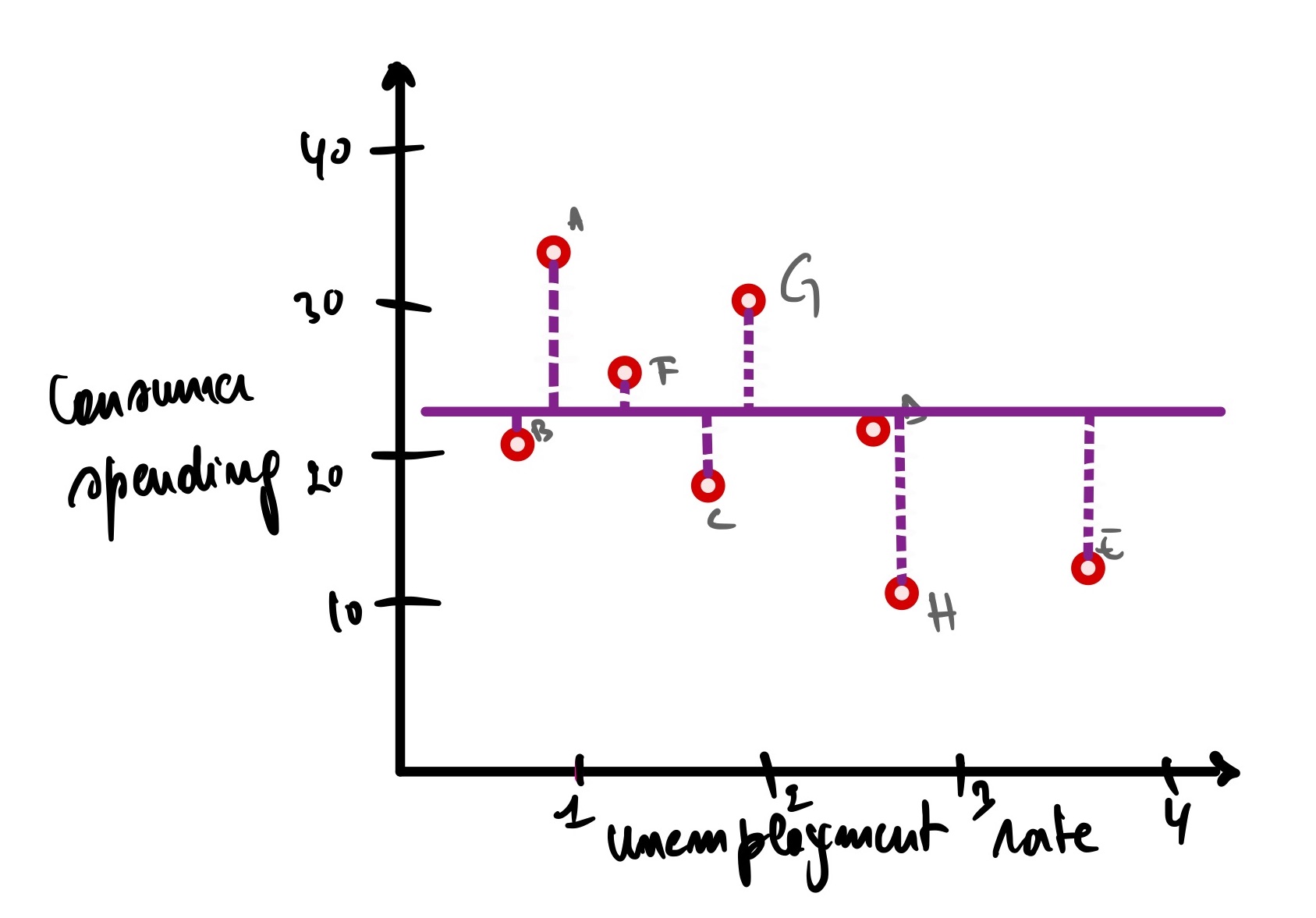
The consumer spending means is 22500, so now the SSE around the mean is equal to

∑(yᵢ - µ)² =

(Ax - µ)² + (Bx - µ’)² + (Cx - µ)² + (Dx - µ)² + (Ex - µ)² + (Fx - µ)² + (Gx - µ)² + (Hx - µ)² =

(34 - 22.5)² + (21 - 22.5)² + (18 - 22.5)² + (23 - 22.5)² + (13 - 22.5)² + (26 - 22.5)² + (31 - 22.5)² + (10 - 22.5)² =

(11.5)² + (-1.5)² + (4.5)² + (0.5)² + (-9.5)² + (3.5)² + (8.5)² + (-12.5)² =

132.25 + 2.25 + 20.25 + 0.25 + 90.25 + 12.25 + 72.25 + 156.25 = 486

Our normal SSE, as previously calculated, is 242

The formula to get R² = SSE(mean) - SSE(line of best fit)/SSE(mean) = (486 - 242)/486 = 244/486 = 0.5

The result is 0.5 (50% reduction in the size) of the errors between the mean and the fitted line. In other words, R² tells us the percentage of errors around the mean shrank when we used the line of best fit. That means the errors have decreased, meaning that the fitted line fits the data better than the mean.

If SSE (mean) = SSE (line of best fit) or if R² = 0, that means that the two models are equally good (or bad), and when SSE (line of best fit) = 1, meaning there has been a 100% improvement of the model. Then the model fits the data perfectly (which is not always a good thing. see overfitting on this post)

Note

• As we mentioned before, R² can be calculated with MSE as well

  R² = [SSE(mean)/n - SSE(line of best fit)/n] / SSE(mean)/n, and by consolidating all the divisions, we have

  R² = [SSE(mean) - SSE(line of best fit)/SSE(mean)] x (n/n) =

  R² = SSE(mean) - SSE(line of best fit)/SSE(mean)

• Those with a background in statistics might wonder if R² is related to Pearson’s correlation coefficient (r). yes, it is.

  The Pearson correlation coefficient measures the strength and direction of the linear relationship between two variables. It ranges from -1 to 1, where -1 indicates a perfect negative linear relationship, 0 shows no linear association, and 1 indicates a perfect positive linear relationship.

  On the other hand, the R-squared ranges from 0 to 1. R-squared is related to the Pearson correlation coefficient because R-squared is the square of the Pearson correlation coefficient (i.e., R² = r²). Therefore, the Pearson correlation coefficient r can be used to calculate R² and vice versa.

It is good that we have all these measurements on how the fitted line matches our data and help us make predictions. But how confident are we in these analyses? How do we know that the fitted line’s slope is the best we can get? Well, the P-value is here to help out answer those questions.

P-value

So what is a p-value? The simplest definition is the measurement of confidence in the results from a statistical analysis. In other words, it tells us the probability that a particular outcome could have occurred by chance or not

Let’s illustrate this with an example: we have countries A and B. We want to know if the population in country A is taller than in country B. We want to know if there is a significant height difference between the two countries. In other words, if the difference between country A’s and country B’s height is not due to random chance.

So we collect the data on the heights of the people in each country, then we find out that in country A, 67% of people are 160cm+ versus 59% in country B are 160cm+. Well, you might conclude that people in country A are taller; there is no doubt about that. Think again; when we are sampling these people, we are not measuring every individual in the country; we make a “sample inference,” which refers to making conclusions about a population based on information collected from a sample, not every individual. So we might have collected maybe the only tallest people in the country for country A and ignored the rest? We might have also sampled the average height people for country B? who knows? We can’t just deduct any concrete conclusion from it.

Note: The more data we collect, the better, but this is not always possible as it can be time and cost-consuming. That is why we take a sample that best represents the whole population.

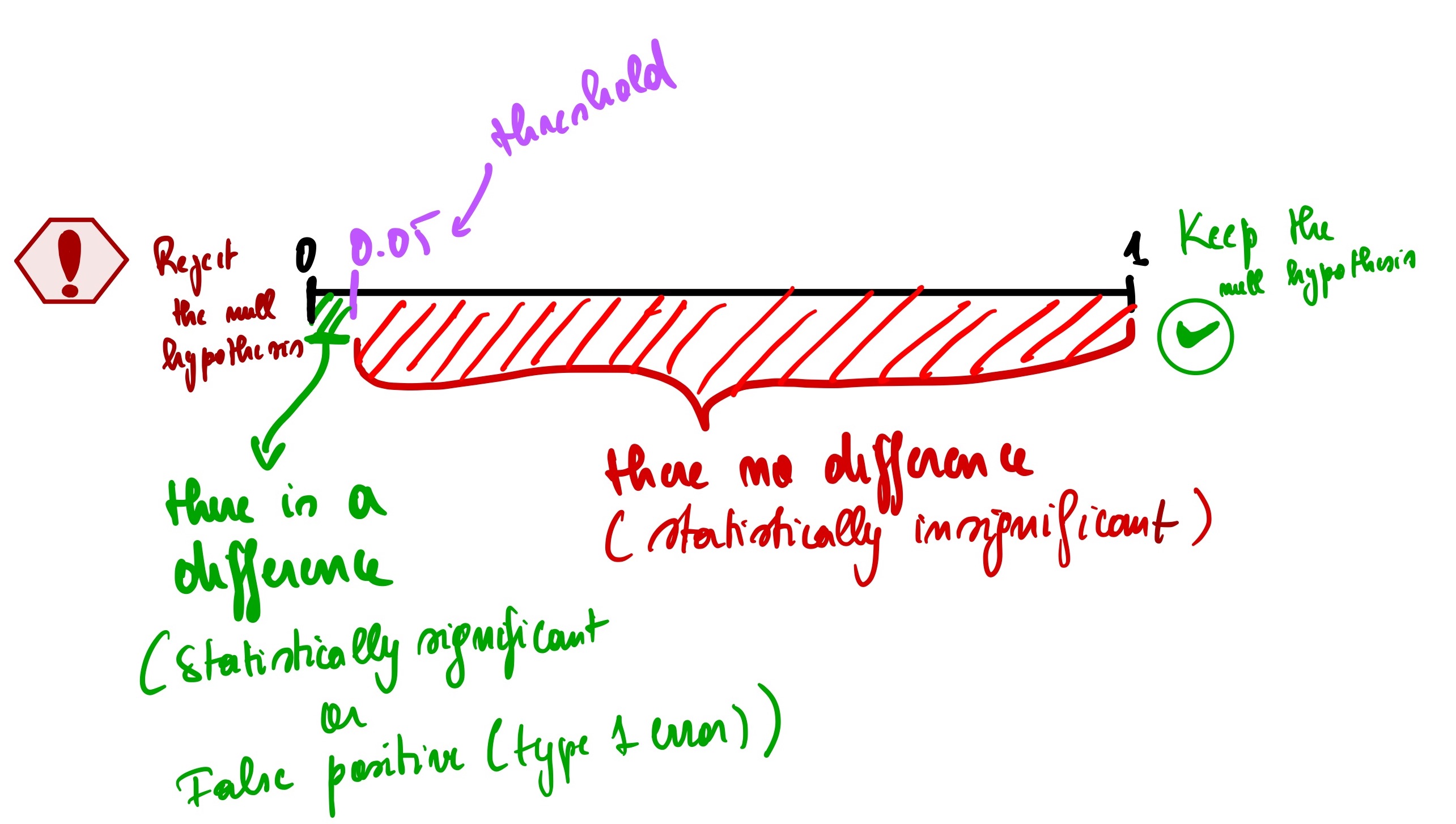
So the p-value helps us to overcome this doubt; p-values range from 0 to 1. The closer the p-value is to 0, the more confident that there is a statistically significant difference between country A and country B population’s heights, meaning the difference is unlikely to be due to chance alone. It is a false positive (Type 1 error).

Now a question arises: how small does this p-value need to be to conclude that there is a statistical difference between country A and country B? in other words, what is the threshold to use? Well, there is a conventional threshold commonly used among statisticians, and it is 0.05. Using our example, if there is no difference between the heights of people in country A vs. B and they had to do the same analysis repeatedly, only 5% of those analyses would result in a bad outcome.

After doing some calculations of the P-value(usually done using a tool like Excel or Python), we found out that the P-value is 0.71, which is greater than 0.05. It means that even though we have a more significant percentage of taller people for country A, it does not necessarily mean that there is a statistically significant difference between people’s height in the two countries.

Note: The threshold of 0.05 is not an absolute threshold; it can vary depending on how confident we want to be with our analysis. For example, if we conduct a study involving human health in the medical field, it is best to use a 0.01 threshold to ensure that we minimize false positives as much as possible. On the other side of the spectrum, we are analyzing which communities in the city are consuming more chocolate then a threshold of 0.2 can do just fine.

Another thing to remember is that the p-value does not tell us how different they are. It only just tells us if there is a difference or not. For example, a p-value of 0.71 (71%) is not much different than a p-value of 0.23 (23%) percentage-wise. It tells us that those two p-values are statistically insignificant when the threshold is 0.05.

Finally, we can’t discuss the p-value without mentioning the null hypothesis. A null hypothesis is a statement that assumes there is no significant relationship at the beginning of an analysis (it is like a “default” position that you start with), meaning that we start the study with the assumption that the P-value < 0.05. After calculating the P-value, we then keep the null hypothesis (when we find no difference) or reject the null hypothesis (when we discover that there is indeed a difference).

Let’s summarize everything discussed in the p-value with this simple illustration below.

How does gradient descent relates to linear regression?

Going back to our previous example of the unemployment rate and consumer spending

Now that we know that R² and P-value mean, we have R² = 0.76 and a P-value = 0.14

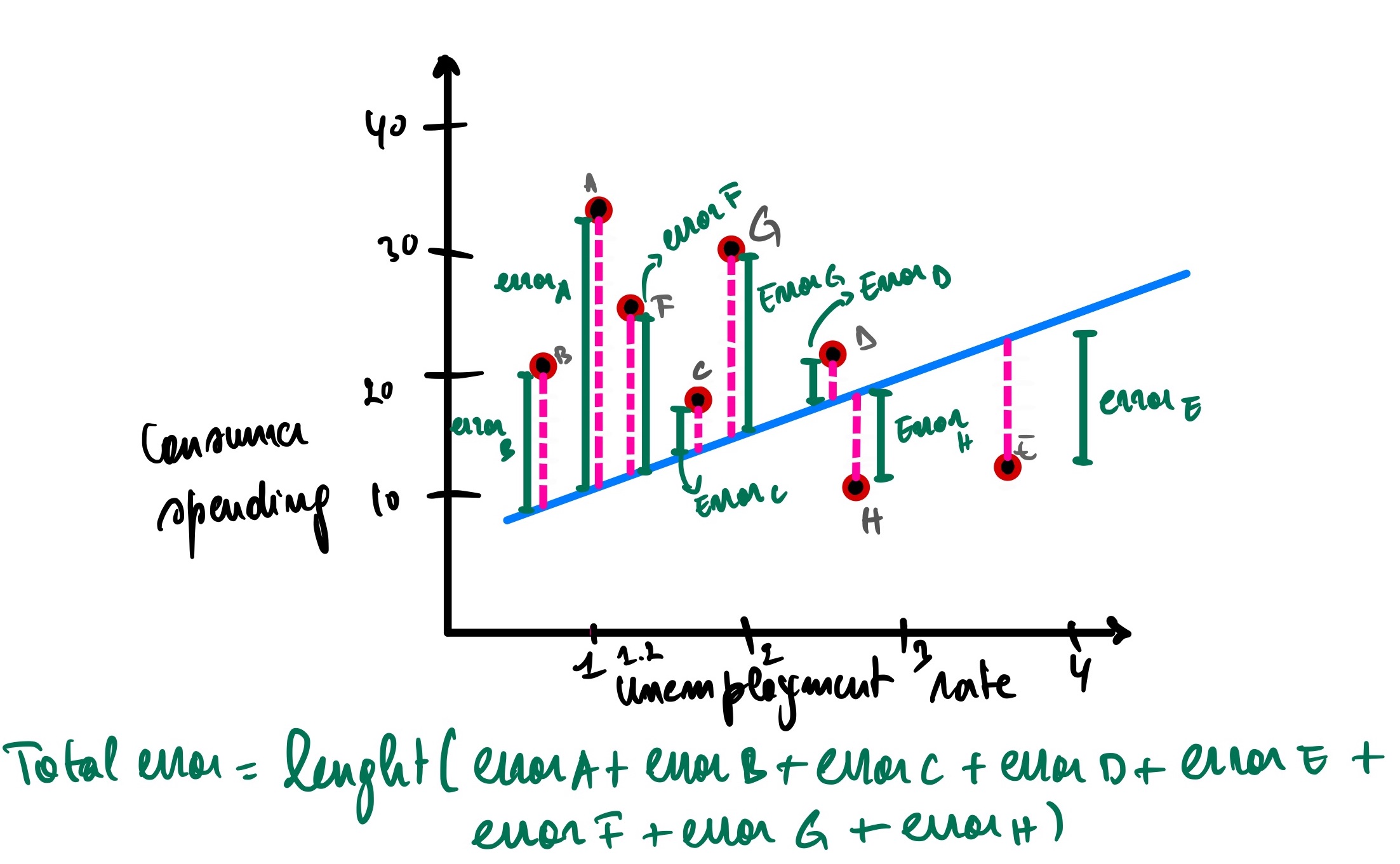
Would this model make good predictions for unseen cities? Of course not. But how can we quantify that this model is worst than the previous one? We can look at the total errors by adding the length of the pink lines, which is the summation of the distance between the observed and predicted data points.

Let’s imagine for a second that we have a new line that fits the data this way.

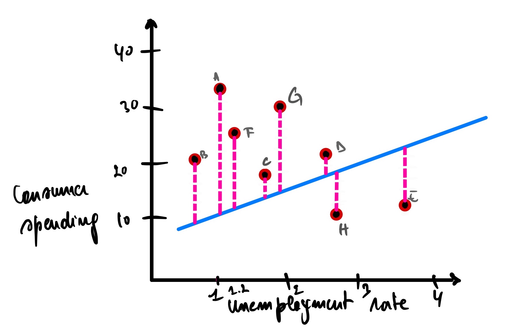
We can see that the total errors (SSE) of the second model that fits our data is greater than the first model, meaning that this second model does not fit our data well compared to our first model. In other words, the second model won’t make a better prediction than the first one.

Now, how about this one?

This one is better than the second model but worse than the first model, meaning that its SSE is less than the second model’s SSE but greater than the first model’s SSE.

Now, how about this one?

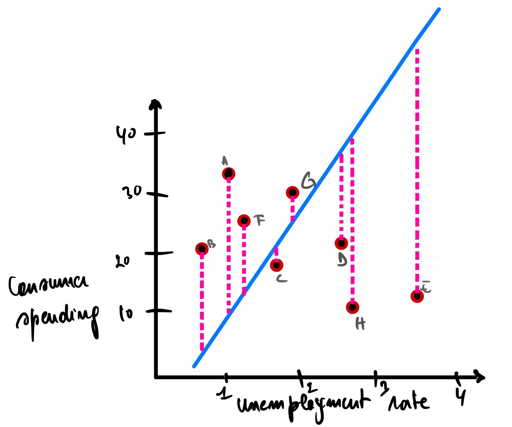
Okay, this one, we can all agree that it is the worst of the bunch.

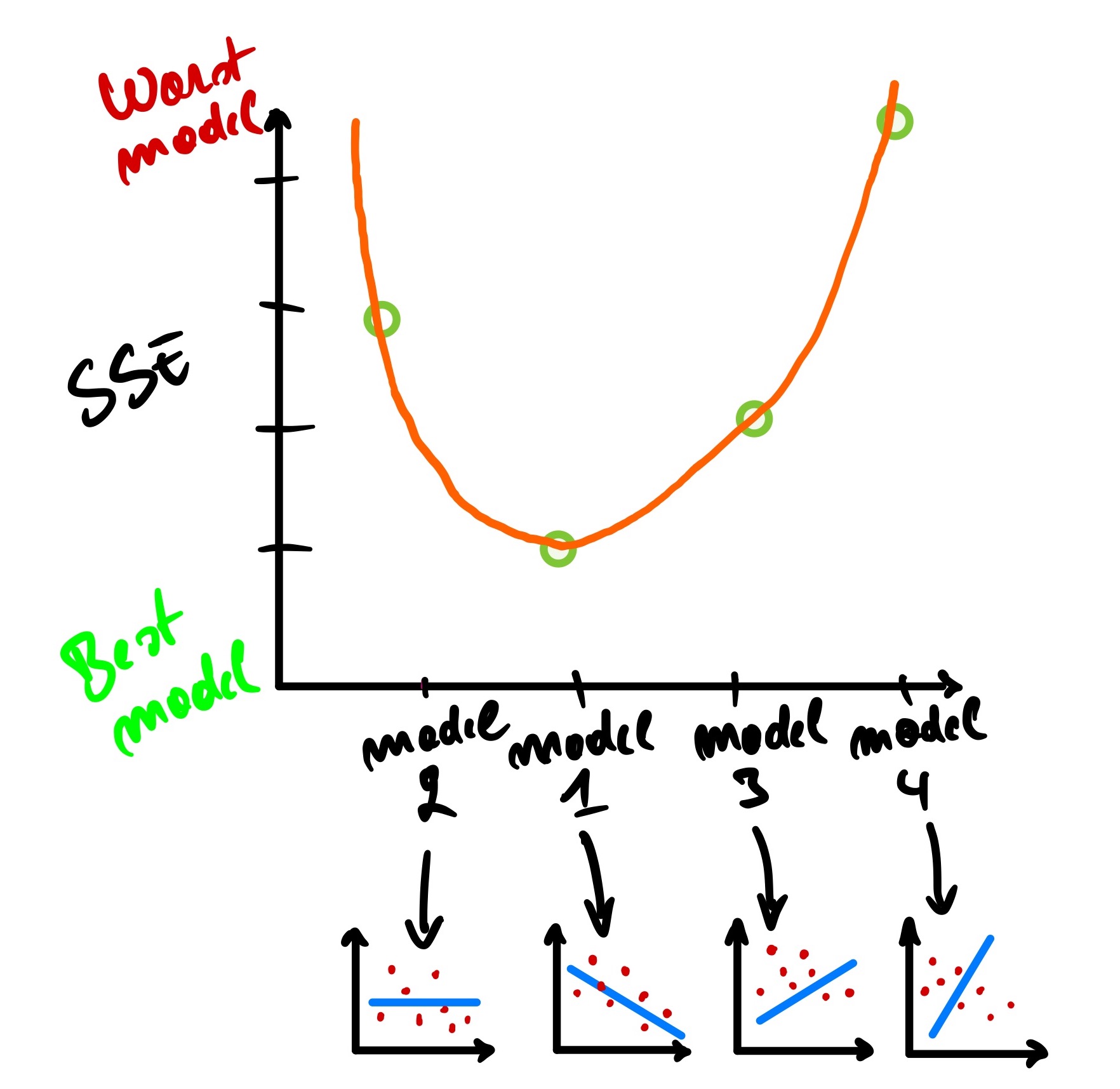
Using this information, we can plot the SSE on the Y-axis of a graph and visualize how the lines perform one again another.

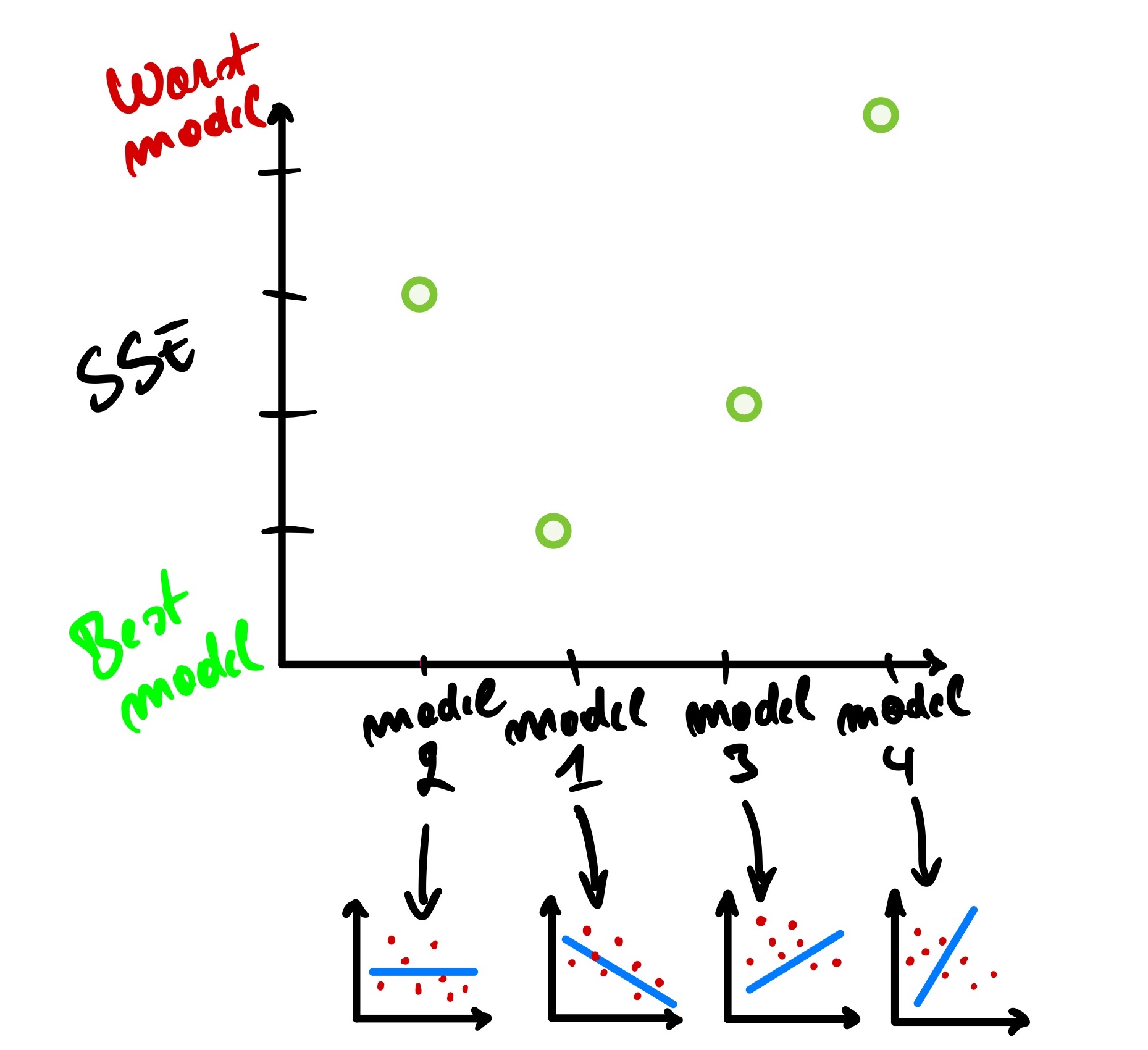
We can see that model 1 has the smallest SSE while model 4 has the largest SSE.

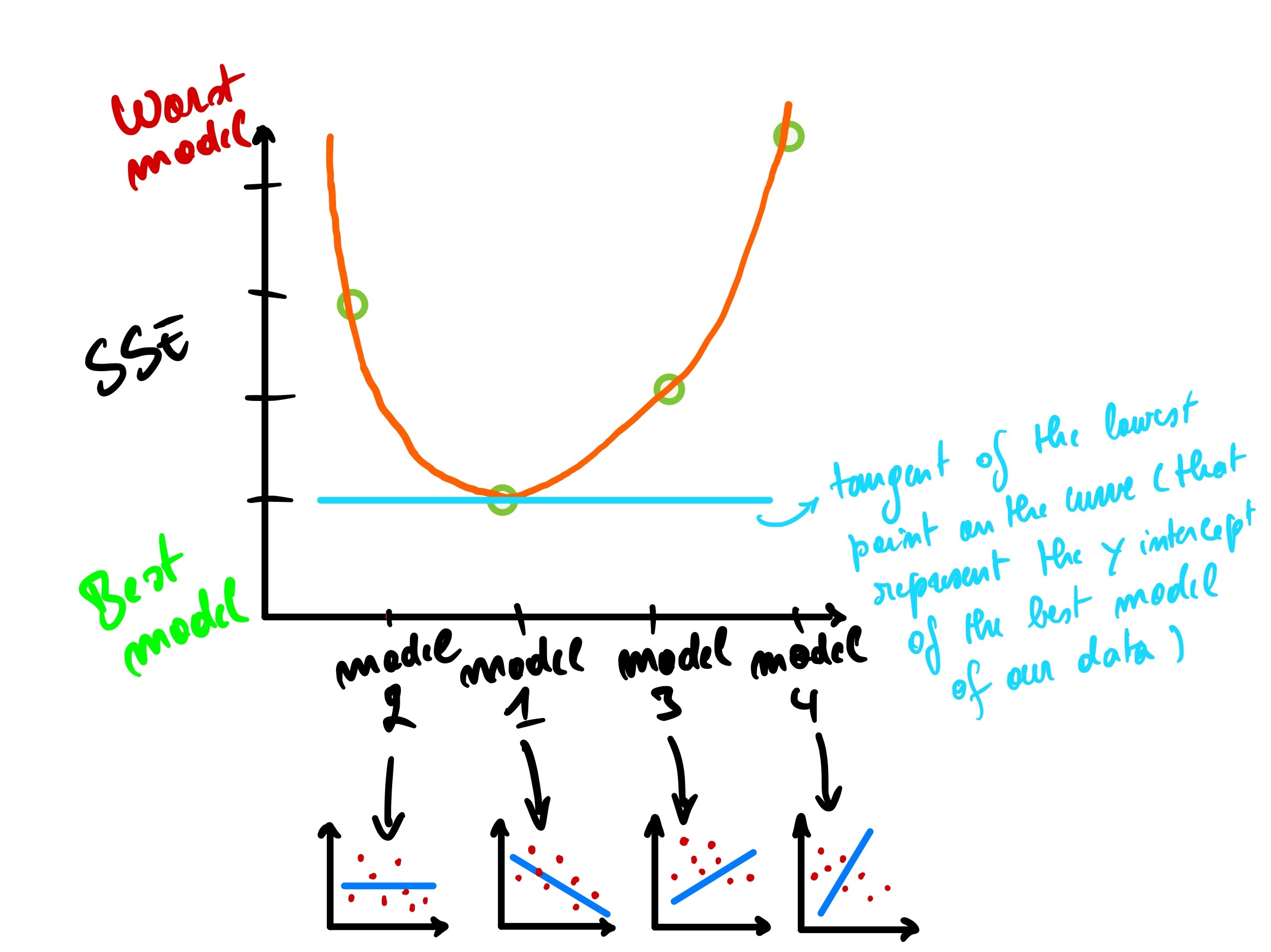
We could plot as the Y-axis intercept of those models, and from there, we can have a curve-like plot.

We can have it animated for a better understanding.

gif credit: https://derekogle.com/

So to find the best model, we need to get to the lowest point on that curve, representing the y-axis intercept of the best model that fits our data. And how do we get that lowest point? Using the derivative of the curve where the derivative is equal to 0; means that the tangent line on that point is horizontal.

Gradient descent is the iterative method to find the lowest point of the curve where we have the minimum error between the actual and predicted values of a machine learning model. It starts with a guess at any point on the curve and then goes on into a loop that improves from the previous guess until it reaches its lowest point. Gradient descent is used not only for linear regression but also for logistic regression, neural networks, and other machine learning models.

Multidimension linear regression

So far, we have seen a linear regression within two variables (two dimension axis). In this case, we only have one independent variable known as input or predictor (unemployment rate) and a dependent variable known as output, response variable, or target (consumer spending). However, this does not mean that it is always this way. We can have multiple input and output variables.

Let’s add another independent variable to the mix, the inflation rate. So now we have two independent variables; as the unemployment rate and inflation rate increase, this should decrease the consumer spending of the people in any given economy. This is called a multidimensional linear regression with 3 axes and a plane instead of a line representing the model.

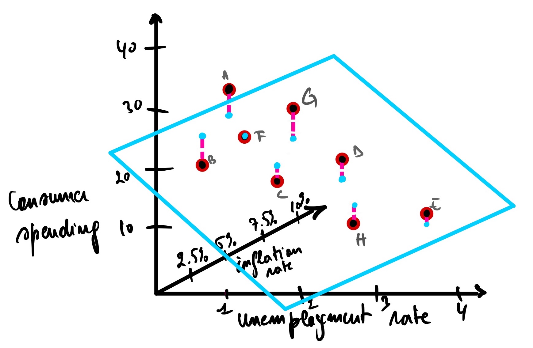
The same concepts apply here; the best model will have a minimum distance between the actual data points and the predicted data points. R², P-value, and gradient descent are all calculated the same.

Note: For instance, when we have more than 3 variables, we won’t be able to represent it on a graph as we just did because we live in a 3-dimensional world, and so far, there is no way to have 4-dimensional representation. But besides this, all the other concepts seen are the same.

Conclusion

As we have seen, linear regression is one of the simplest Machine Learning models, yet it is very powerful. Depending on the problem we are trying to solve, this might be what we are looking for, as simplicity is a desirable model feature when we want to understand how a model came up with the result (model interpretability). For example, when a model is used for loan underwriting, we need to understand what independent variables contributed the most to granting or rejecting a loan application. It is also instrumental in the medical field when high stake accountability is involved. Neural networks provide better results but might not be the best because they lack interpretability. That is why it is commonly referred to as a black box model.

In this post, we explored the main topic of Linear regression; we defined what it is, when to use it, how it works, and all its metrics and variation. We have covered almost any theory you need to know about linear regression, and I hope you learned something new as I did when writing this blog. I also discovered the power of ChatGPT in improving my productivity while learning and writing. I will certainly use it for my next blog post, a hands-on version of this post where we will dive into linear regression using the scikit-learn library. Excited about that one, so stay tuned!

If you like this post, please subscribe to stay updated with new posts, and if you have a thought, correction, or a question, I would love to hear it by commenting below. Remember, practice makes perfect! Keep on learning every day! Cheers!

Share this post on