Welcome back! I am very excited about this post as we are introducing machine learning and its commonly used jargon. You will have a broad overview of machine learning, how it works, and even write our first machine learning code at the end of the post. To understand advanced machine learning, we first need to have a good grasp of the fundamentals. That is why I think this is the most important post on this blog so far.

With no further due, let’s get started.

1. What is machine learning, and how can a machine learn?

1.1 What is machine learning

Machine learning is a subfield of computer science that studies the ability of a computer to learn and exhibit cognitive abilities without being explicitly programmed.

1.2 How do computers learn?

As we have previously said, computers learn through data. The more the data, the better. Computers are very good at discovering not immediately apparent patterns within a large dataset (tabular or non-tabular) than humans. It is called data mining. Data mining is a whole separate computer science field on its own.

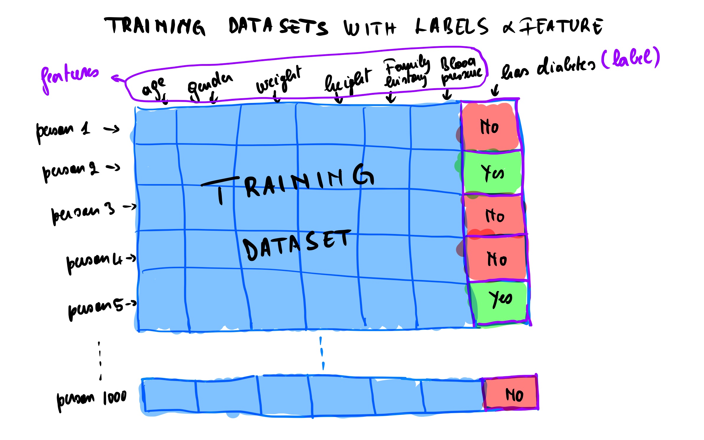
Going back to our question, how can machines learn? one way is by breaking the dataset into two datasets. A training dataset and a testing dataset. As a good rule of thumb, the training dataset should account for 80% of the dataset, and the test dataset should be 20% (more on this later in the post). Each unit of information in the dataset is a datapoint represented as the entire row in a tabular dataset.

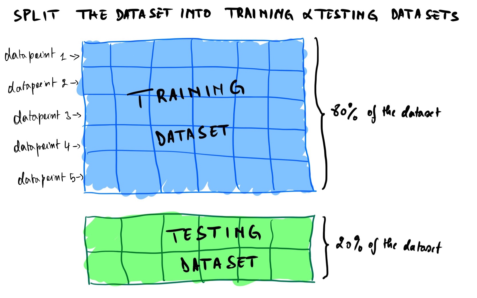
A training dataset is a dataset used to train(teach) the model (also called estimators in Scikit-learn library, and I’ll be using those two words interchangeably). We use the testing dataset to evaluate the model and see how well it has learned (also called measuring its accuracy).

Note: we should never train a model on the testing dataset, or else it defeats the whole purpose of evaluating the model.

Let me explain this statement further. Let’s say you are a student enrolled in a math course. To pass the exam, you have to practice by doing many exercises to become good at it. If the lecture decides to give you the exam paper for practice, probably during the exam time, you will score close to 100%. But does that mean that you have mastered the course? Of course not! You have just memorized the whole exam without really understanding anything. The same happens to a machine learning model trained and tested on a testing dataset. It is called overfitting (more on this later in the post). That is why we need to hide the model from the testing dataset and only train on the training dataset.

2. Use of machine learning VS traditional programming?

To understand when shall we use machine learning, we need first to understand how machine learning and traditional programming work under the hood.

2.1 How machine learning works VS traditional programming?

2.1.1 Traditional programming

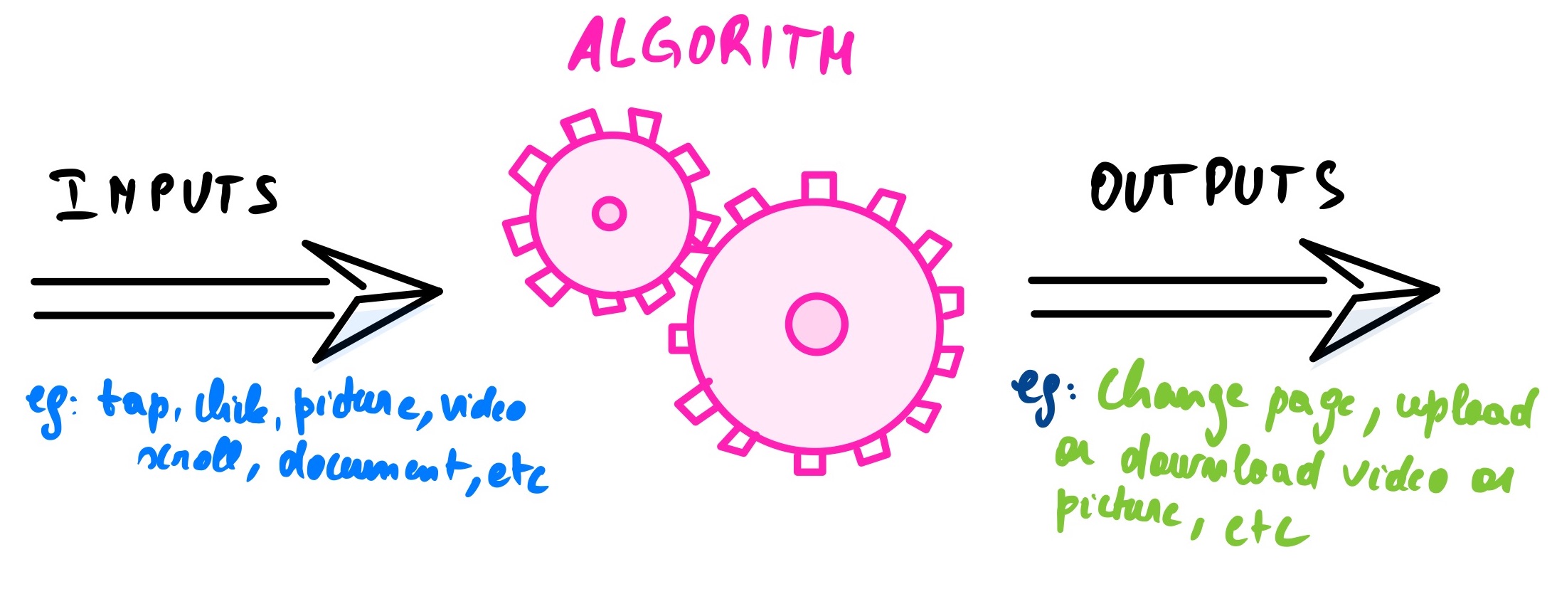
Let’s start with traditional programming. It includes all the backends development, front-end development, mobile development, dev-ops, systems architecture, etc. All these computer science subfields share the same fundamentals of using a set of instructions called Algorithms written by a programmer that takes an input and produces an output. Think of it as a more complex “if and else statement” for example, if a user presses this button, then change the webpage to this new page.

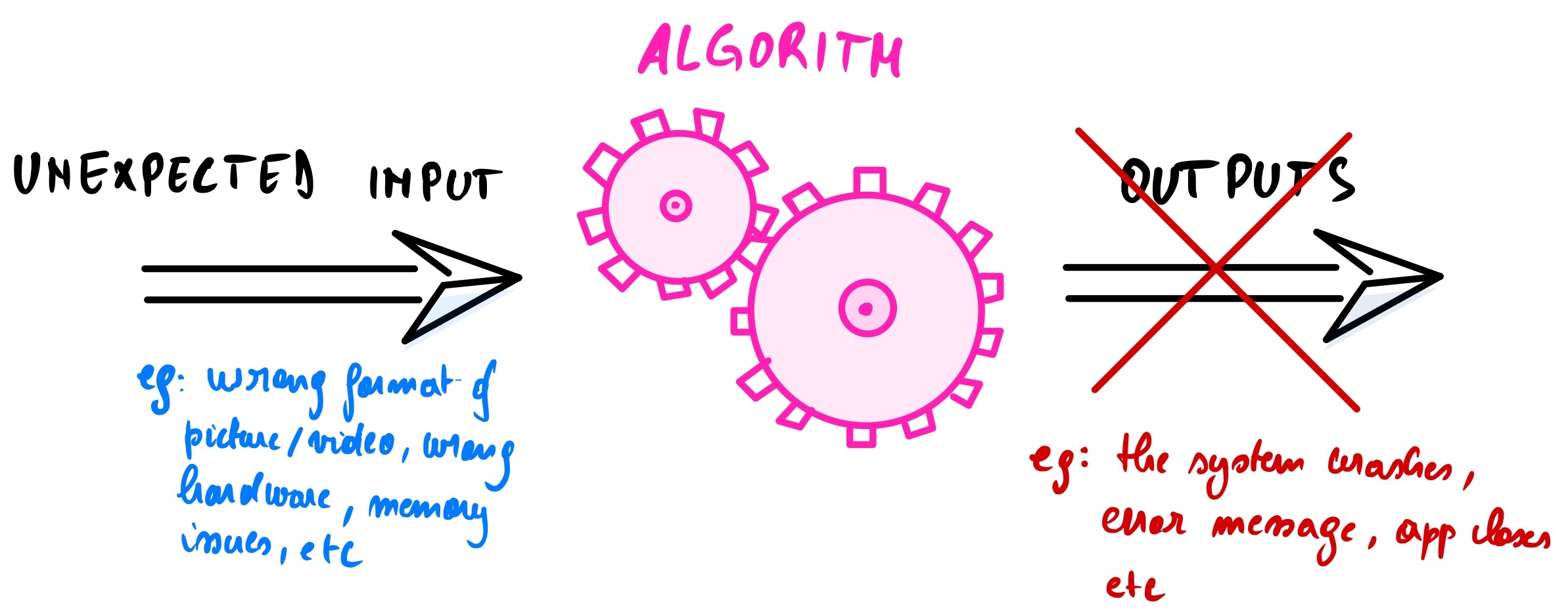
If an unexpected event occurs (not coded), the algorithm will not execute, and the software/app will crash. Now you know what is happening when you see a blue screen in Windows or your mobile app has unexpectedly stopped working. The algorithm can’t troubleshoot itself without the intervention of the programmer. That is why you always have to upgrade your software or app to fix the “bugs”.

2.1.1 Machine learning

On the other hand, machine learning works differently than traditional programming. We feed (train) the machine learning model datasets as input and let the model predict the best output. We, the programmers, don’t explicitly write those instructions. We help the model fine-tune its parameters (more on this later) to find the best predictions. Consequently, the more the data we feed to the model, the better the predictions become overtime.

We evaluate the model and see if it has learned well. If the result is satisfying, then we lunch the model into production. If not, we then analyze the model, fine-tune its parameter, and retraining the model is required.

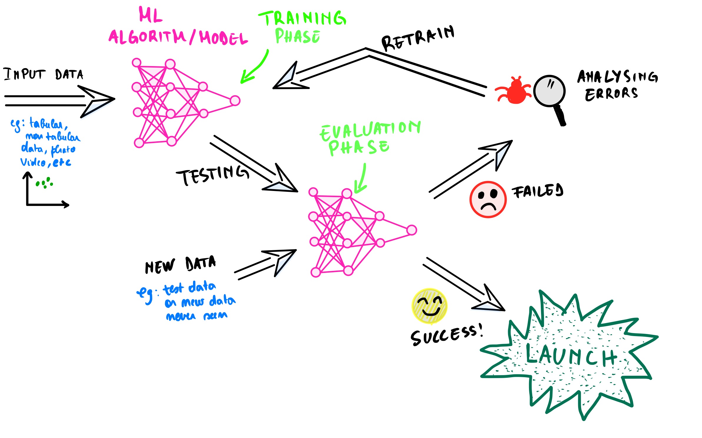
Note: it is crucial to feed the model accurate and clean data (without outliers or missing data) because if you don’t, then the predictions will be off, and its accuracy won’t be reliable. That is why modeling (the process of training the model) is the least consuming task in an end-to-end machine learning project compare to data cleaning. I wrote in this post that data scientists spend 60% of their time cleaning the training data and only 4% modeling and training the model.

2.2 When shall we use machine learning or traditional programming?

Here are some questions to ask yourself when deciding to use whether machine learning or traditional programming for a project:

• Does this project try to solve a problem that requires a lot of fine-tuning and rules? If you answered yes, then use machine learning.

  To clarify the point above, let’s say that you work at a bank as a fraud expert analyst, and your boss tells you that there has been a sharp increase in credit card frauds this month. As a fraud expert with programming skills, you need to find a solution to this as soon as possible. You first analyze the transactions reported as fraudulent. You notice interesting similarities among 80% of them: First, those transactions are orchestrated from overseas. Second, they are below one thousand dollars. Third, the account holders are mostly seniors (65 years old and above).

  After gathering these pieces of information, you decided to create a script to detect and block automatically similar transactions that will occur in the future. The code is not perfect, as there are false positives, but after deploying the script for a week, there is a drop in the number of fraudulent transactions reported. Yes! We did.

  After two months, your boss comes back to you and tells you that the number of fraud has gone up again. It seems like the scammers now use a VPN as the transactions appear to be from within the country. Secondly, in the new fraudulent transactions, the amount transacted is not below on thousand dollars all the time. The scammers have found a way to bypass the script that you have put in place.

  Now, you are thinking about two options: Option 1, rewrite a new script with the new rules and option 2, come up with a script that can adapt to new rules without being explicitly coded.

  The first option is tedious, and it is a matter of time until the scammers find another way of going around it. So the best option would be option 2, to let the script adapt and block the fraudulent transactions with minimal intervention.

• Does this project try to solve a complex problem where using traditional programming has failed? Then use machine learning. Example: Detection of a cancer cell in an image.

• Does this project try to solve a complex problem in a constantly changing environment? Then use machine learning as it can adapt to a constantly changing environment as it receives more and more data. Example: Robots that sort trash on a recycling line depending on the type of materials using computer vision.

• Does this project try to solve a complex problem with a large amount of data? Then use machine learning. Example: Self-driving cars in a busy street.

I firmly believe that machine learning and traditional programming will continue to co-exist as they solve problems differently. Therefore one can’t replace the other.

3. Types of machine learning

There are different types of machine learning systems depending on how we train them, how they learn, and how they generalize.

3.1 Types of machine learning system classified on how we train them

3.1.1 Supervised learning

We train these types of machine learning using labels. It means that in the training dataset, we have the desired outputs. We use different datapoints attributes called features or predictor to train the model and predict the labels.

For example, given a dataset with features like age, gender, weight, height, family history and blood pressure, we are trying to predict if someone has diabetes or not. The last column in the training dataset is the label. This type of training is called classification model because we are classifying the data points into two groups (has diabetes or does not have diabetes).

The labels can also be numerical. In this case, we are dealing with a regression model. An example of this would be predicting the houses price depending on different features like the size, the location, the mortgage interest rate, etc.

3.1.2 Unsupervised learning

For this type of machine learning, we train the model without labels. With your help, the model will try to figure out the correlations within the datasets. Listed below are the unsupervised tasks we could perform:

• clustering to discover similar data points within the dataset and hierarchical clustering to group similar data points into smaller groups. Each group is called cluster

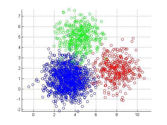Credit: Kdnuggets

• dimensionality reduction to merge similar features into one feature. For example, we could combine the smartphone’s age with its battery health as those two are strongly correlated. We call it feature extraction

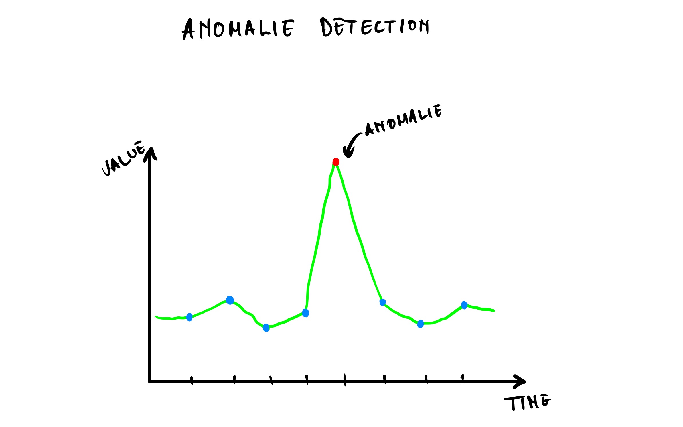
• anomaly detection by detecting automatically and removing outliers (a data point that differs significantly from the rest of data points) and novelty detection by detecting but not flagging as outliers incoming data point that looks different from the rest of data points in the dataset.

• association rule learning to discover underlying relations between data points in a large dataset. For example, through data, we have found out that clients in the supermarket who bought chicken will most likely buy the barbeque sauce. It makes sense to give a bundle pricing discount or place those two products close together on the shelves to incentivize the purchase.

3.1.3 Semisupervised learning

We can combine a small labelled dataset and an unlabeled dataset to get a semi labelled dataset. Now you might ask why can we just label the whole dataset? well because labelling a dataset is time-consuming and very expensive as it does require a skilled person.

Semisupervised learning is a great alternative from supervised learning because some machine learning models are able to train using a partially labelled dataset.

3.1.4 Reinforcement learning

Reinforcement learning works differently than the previous types. It involves an “agent” taking action to perform tasks using a strategy called “policy”. We want him to do one specific task and avoid the others. Each time the agent accomplishes the desired task, he gets rewarded. If not, he gets penalized.

The more the rewards, the more the agents understand that it needs to perform the desired task (just like the Pavlov’s dogs conditioning). Through trials and errors with the feedback (in terms of rewards and penalties), the agent learns and becomes good at the task we require him to perform.

Of course, this is a simple explanation of reinforcement learning as it is a bit more complex, but you have at least a basic understanding. Deepmind’s AlphaGo used reinforcement learning to beat the professional Go player Lee Sedol in 2016.

Jabril has a video where he did a great job at explaining reinforcement learning in details. By the way, I highly advise watching his entire AI crash course series.

3.2 Types of machine learning system classified on how they learn

3.2.1 Batch learning

For this type of learning, the model has to be trained one step at a time. It means that the model can’t learn continuously on the fly. It needs first to train with all the available data before the initial deployment into production. Once into production, it will only predict using the training dataset we had previously used.

To retrain the model on new data, we need to take down the model, train a new version of the model with the full dataset (old and new) offline, then replace the old model and deploy the new version. That is why it is called offline learning. The con of this method is that it is time and resource consuming.

3.2.2 Online learning

Here, the model is train gradually, meaning that we can feed the model new data in small groups (called mini-batches) on the fly while the model is in production. This method is way cheaper than batch learning. The disadvantage is when the new data quality deteriorates, it also affects the model’s performance. Thus, constant monitoring of the quality of new data is required.

3.3 Types of machine learning system classified on how they generalize (making a prediction on new data)

3.3.3 Instance-based learning

This type of learning is comparable to the script used for spotting the fraudulent transactions seen above. That script looked at the similarities (overseas transactions below $1000 and senior account holder) among the reported fraudulent transactions and new transactions, then flagged the very similar ones.

This script learnt by examples, by memorizing the similarities and made predictions on new data it has never seen before.

3.3.4 Model-based learning

As the name implies, model-based learning means that we build and use a model to make predictions. Let’s illustrate this with a concrete example.

We all have heard the expression: “Money does not buy happiness”. As an avid researcher, you want to prove that with numbers, and as we know: “Numbers don’t lie”. Right?

So you decide to survey your friends, family members and internet users, asking them their incomes and then rank their happiness in life on a scale of 1 to 10.

You got a total of 498 responses, which is not a large dataset, but for this experiment, it is a good population sample. Download the dataset here.

Let’s first start by importing Numpy, Pandas, Matplotlib and the CSV file.

import numpy as np
import pandas as pd
import matplotlib.pyplot as plt
%matplotlib inline

income_data = pd.read_csv("income_data.csv")
income_data

	Unnamed: 0	income	happiness
0	1	3.862647	2.314489
1	2	4.979381	3.433490
2	3	4.923957	4.599373
3	4	3.214372	2.791114
4	5	7.196409	5.596398
...	...	...	...
493	494	5.249209	4.568705
494	495	3.471799	2.535002
495	496	6.087610	4.397451
496	497	3.440847	2.070664
497	498	4.530545	3.710193

498 rows × 3 columns

Now, let’s drop the Unnamed: 0 column because it is a duplicate column since we already have the index column automatically added by pandas. Let’s also scale up the income column to 10000 to make it more realistic and round the numbers in the dataset by two decimal places.

income_data = income_data.drop(columns=["Unnamed: 0"])

income_data["income"] = income_data["income"] * 10000

income_data = income_data.round(2)

income_data

	income	happiness
0	38626.47	2.31
1	49793.81	3.43
2	49239.57	4.60
3	32143.72	2.79
4	71964.09	5.60
...	...	...
493	52492.09	4.57
494	34717.99	2.54
495	60876.10	4.40
496	34408.47	2.07
497	45305.45	3.71

498 rows × 2 columns

Then, let’s plot the dataset on a scatterplot.

plt.scatter(income_data["income"],income_data["happiness"], alpha=0.5,edgecolors="black")
plt.xlabel("Income")
plt.ylabel("Hapiness scale")
plt.show()

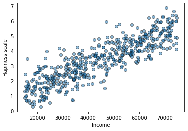
Yeah seems like the more money we make, the happier we become! On average, someone making over 70000 dollars is likely to be happier than someone making 20000 dollars. Shocking right?

We can see that the data points follow an upward direction. Now let’s try to create a model that follows best those data points. This step is called a model selection, and in this example, it will be a linear model also called linear regression since there are no curves in the upward direction.

The formula is as follow called the population regression function:

$\alpha$ = $\theta_{0}$ + $\theta_{1}$ $\times$ $\lambda$ + $\epsilon$

where

$\alpha$ is the predicted value. In this case, the happiness scale.

$\theta_{0}$ is the first parameter called intercept of the predicted values $\alpha$ (happiness scale).

$\theta_{1}$ is the second parameter called regression coefficient.

$\lambda$ is the independent variable. In this case, it is the income.

$\epsilon$ is the error(different from the sample error e), also called margin error in our prediction of the regression coefficient. In our case, we assume that there is no error implying that $\epsilon$ = 0

To keep it simple, we will rewrite the equation as follow:

happiness scale = $\theta_{0}$ + $\theta_{1}$ $\times$ income

Note: if you have taken a high school algebra course, you might have recognized this formula as the equation of a straight line y = mx + b where x and y are the x and y axis coordinates, m is the slope of the line and b is the y intercept.

This model has two parameters $\theta_{0}$ and $\theta_{1}$. We need to find those two parameters value to define a line that follows the best data points. How do we find that? We have the choice between two functions. The utility function(also called fitness function) and the cost function. So what is the difference and which one should we use? The short answer is it depends.

The utility function measures how good the model is, and the cost function calculates how bad the model is. Since we are dealing with linear regression, it is best to use the cost function to compare the distance between the predicted data point coordinate and the linear regression line. We need to reduce that distance as much as possible. The shorter that distance, the more accurate is our model.

So how do we get that linear regression line to best align with the data points? We use the scikit-learn functions to find the two parameters $\theta_{0}$ and $\theta_{1}$. This is what’s called training the model.

We import directly the function from the scikit-learn library.

from sklearn import linear_model

Then, we store the estimator (this is how we call a model in the scikit-learn library) in the est variable.

est = linear_model.LinearRegression()

Now we store the features as a one-dimensional array in Xsample_inc and Ysample_hap using the c_ Numpy function.

Xsample_inc = np.c_[income_data["income"]]
Ysample_hap = np.c_[income_data["happiness"]]

the linear model estimator learn from those data points using the fit function

est.fit(Xsample_inc,Ysample_hap)

LinearRegression()

Finally, we access the values of $\theta_{0}$ (the intercept) and $\theta_{1}$ (regression coefficient) by calling the intercept_ and coef_ functions on the estimator.

est.coef_[0][0]

7.137623851143422e-05

o0,o1 = est.intercept_[0], est.coef_[0][0]

print("the intercept 𝜃0 is {} and the regression coefficient 𝜃1 is {}".format(o0,o1))

the intercept 𝜃0 is 0.20472523776933782 and the regression coefficient 𝜃1 is 7.137623851143422e-05

With these two values, we can plot the linear regression line.

plt.scatter(income_data["income"],income_data["happiness"], alpha=0.5,edgecolors="black")
plt.axis([15000,75000,0,7.2])
X_coordinate = np.linspace(15000,75000)
plt.plot(X_coordinate, o0 + o1*X_coordinate, color="r",linewidth=3)
plt.text(18000,6.5, r"$\theta_{0} = 0.20$",fontsize=14,color="r")
plt.text(18000,5.5, r"$\theta_{1} = 7.13 \times 10^{-5}$",fontsize=14,color="r")
plt.xlabel("Income")
plt.ylabel("Hapiness scale")
plt.title("Linear regression of Hapiness VS income")
plt.show()

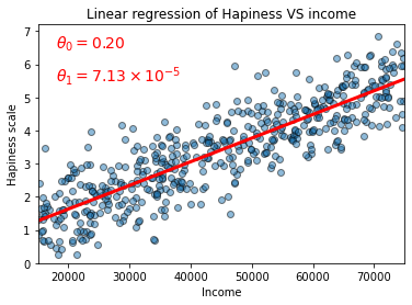
We plot the dataset’s features using a scatter plot and set the plot axis limits. We then create an interval X that represents the axis limit of the linear regression line and set it to range from 15000 to 75000 (we don’t need the steps because drawing a line requires only two coordinate in a 2D dimension).

We then plot X_coordinate on the X and Y axis using the linear equation and change the color of the line to red using the character "r".

Finally, we place the text of $\theta_{0}$ and $\theta_{1}$ in the plot with the axis labels and title.

If we don’t need the values of $\theta_{0}$ and $\theta_{1}$ and only want to plot the linear regression line seaborn has a function for that.

import seaborn as sns

sns.regplot(x=income_data["income"],y=income_data["happiness"],line_kws={"color":"red","linewidth":3},scatter_kws={"alpha":0.5,"edgecolor":"black"})
plt.text(18000,6.5, r"$\theta_{0} = 0.20$",fontsize=14,color="r")
plt.text(18000,5.5, r"$\theta_{1} = 7.13 \times 10^{-5}$",fontsize=14,color="r")
plt.title("Linear regression of Hapiness VS income")
plt.xlabel("Income")
plt.ylabel("Hapiness scale")
plt.show()

Now comes the fun part, prediction time! Let’s predict the happiness scale of a new person (not from our survey) given his income. Let’s say person A makes per year $61200.

We have 2 ways of predicting the happiness scale:

1. Using the formula happiness scale = $\theta_{0}$ + $\theta_{1}$ $\times$ income.
2. Using the model’s predict function (most recommended).

1. Using the formula

Using the equation that we previously saw:

happiness scale = $\theta_{0}$ + $\theta_{1}$ $\times$ income

After replacement with the numerical values, we get:

happiness scale = 0.2047 + 7.13 $\times$ $10^{-5}$ $\times$ 61200

happiness scale ~ 4.56

2. Using the model’s function

Now let’s calculate this in codes, shall we?

personA_inc = 61200

personA_hap = est.predict([[personA_inc]])[0][0]
print("The estimated happiness scale of person A with an income of ${} is {:.2f} using linear regression.".format(personA_inc,personA_hap))

The estimated happiness scale of person A with an income of $61200 is 4.57 using linear regression

We call the predict function on the estimator then pass as an argument the person A’s income. Note that we add the indexes selection [0][0] because the predict function accepts only an array-like or matrix as an argument.

Now, let’s plot this.

plt.scatter(income_data["income"],income_data["happiness"], alpha=0.5,edgecolors="black",zorder=1)
plt.axis([15000,75000,0,7.2])
X_coordinate = np.linspace(15000,75000)
plt.plot(X_coordinate, o0 + o1*X_coordinate, color="r",linewidth=3)
plt.text(18000,6.5, r"$\theta_{0} = 0.20$",fontsize=14,color="r")
plt.text(18000,6.0, r"$\theta_{1} = 7.13 \times 10^{-5}$",fontsize=14,color="r")
plt.xlabel("Income")
plt.ylabel("Hapiness scale")
plt.title("Linear regression of Happiness VS income")

# Prediction data point
plt.vlines(personA_inc, 0, personA_hap,linestyles="dashed",linewidth=3,colors="k")
plt.hlines(personA_hap, 0, personA_inc,linestyles="dashed",linewidth=3,colors="k")
plt.scatter(personA_inc, personA_hap,c="k",marker="o",s=100,zorder=5)
plt.text(15500,4.7, "prediction = 4.57",fontsize=12,color="k")
plt.text(62000,0.2, "$61200",fontsize=12,color="k")

plt.show()

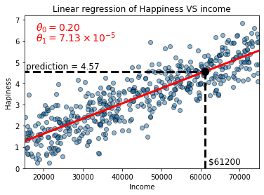
We can predict the happiness scale using the plot by drawing a perpendicular line (also called the projection of a point to a line) from the X-axis coordinate (61200) to a point belonging to the linear regression line. From that point, we draw another parallel to the X-axis projected to the Y-axis. That point on the Y-axis is our prediction.

Sweet! Now that we understand how we drew the dashed lines, let’s go back to the codes.

We have already seen the first nine lines of codes, and we will focus on the following lines of code. We use the Matplotlib’s vline function to project personA_inc value to the linear regression line passing as argument the personA_inc value as X, 0 and personA_hap to draw a line parallel to the Y-axis starting from the value of personA_hap on the X-axis. We set the linestyles to dashed to draw a dashed line, increase its width by three and finally change the color to black using k. Vice versa for the hline.

To emphasize the projected point where the income and the happiness scale meet on the linear regression line, we increase its size, setting the color to black and zorder to 5 (because we want that point to be on the top of the linear regression line).

How about we use instance-based learning instead of model-based learning? For this, we could use a simple model called K-nearest neighbors. We will look at this estimator in the upcoming post but for now, what you need to know is that it uses the features of the nearest data points(the neighboring points)to make predictions, thus the name.

The code is almost the same as model-based learning. The difference is that we are using a different estimator. Instead of using linear_model we use KNeighborsRegressor.

Note: we are importing a regressor model and not a classifier because we are predicting a number.

from sklearn.neighbors import KNeighborsRegressor

est_reg = KNeighborsRegressor(n_neighbors=3)

n_neighbors is set to three because we want to predict the scale using the three nearest data points.

est_reg.fit(X=Xsample_inc, y=Ysample_hap)

KNeighborsRegressor(n_neighbors=3)

Now let’s predict and see what we get.

personA_hap = est_reg.predict([[personA_inc]])[0][0]
print("The estimated happiness scale of person A with an income of ${} is {:.2f} using KNN".format(personA_inc,personA_hap))

The estimated happiness scale of person A with an income of $61200 is 4.53 using KNN

We got a result very close to what we got while using model-based learning. Hopefully, you were able to get predictions closed to these results.

If these models are deployed into production and don’t perform well, we can do the following:

• add more features like heath status, community vitality, city of residence, life purpose.
• get better quality training data.
• select more advanced and powerful models.

The examples above are basic machine learning projects, but it gives us a climbs into the steps taken for every machine learning projects:

1. We import and clean the data.
2. We select the appropriate model (estimator).
3. We train the model on the training dataset.
4. Finally, use the newly trained model to make predictions on data it has never seen before.

Since there are so many models, how do we choose the right one for our project? Well, the amazing team from the Scikit-learn organization came up with this chart below.

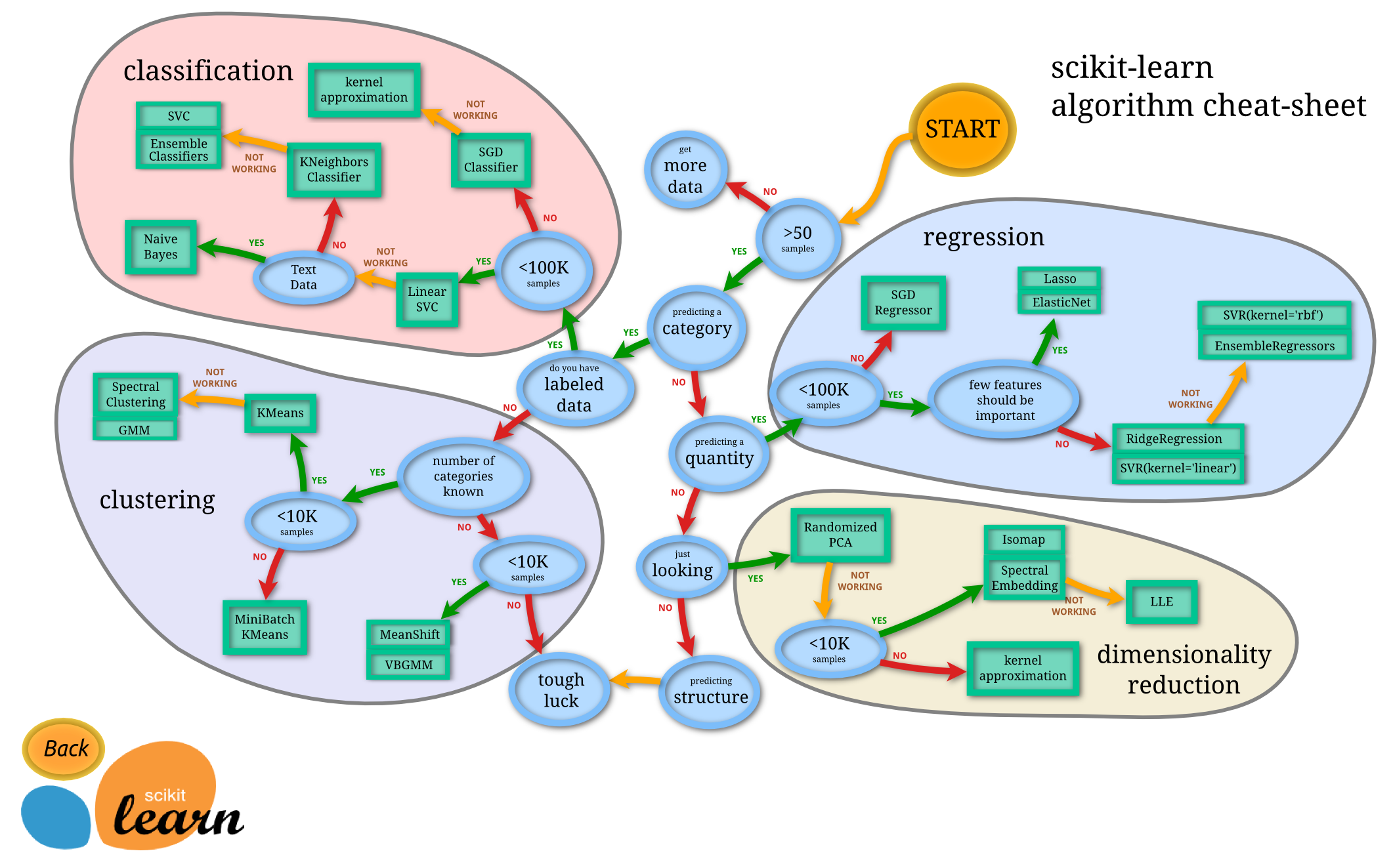
We will be working with some of these models in the upcoming posts, and we will be referring to this diagram frequently.

4. Main challenges of machine learning and how to overcome them

Since we don’t live in a perfect world, machine learning has its own set of challenges caused by the data and the model.

4.1 Challenges related to data

4.1.1 Not enough data

Machine learning requires a lot of data to generalize well on unseen data. Typical machine learning projects require thousands of data points, but more complex projects like self-driving cars will require millions or even billions of data points.

That is why it is challenging and expensive for startups to compete with unicorns like Google, Amazon or Telsa, as those companies already have petabytes of data.

Solution: To get more data

4.1.2 Train on nonrepresentative data

If a model is training on nonrepresentative data, it will come up with biased predictions. Think of this as training on a sample of similar data points, which don’t reflect the whole population. We are training on a small dataset not inclusive of all the possible data points in the population. We call this sampling noise.

The opposite can also true when we have a large dataset, but the sampling methodology used is flawed and inclusive of all the possible data points. We call it sampling bias. It applies to both instance-based and model-based learning.

Solution: Gather more representative data

4.1.3 Train on inaccurate data

It makes sense that a model fed with a dataset full of errors and outliers will not find patterns and generalize on new data. That is why it is always wise to do an exploratory data analysis and data preparation before training the model.

Solution:

1. Identify and remove outliers from the dataset
2. For missing data, we can remove the feature, the data points, replace the missing data with the median or train one model with the feature and one model without it.

4.1.4 Irrelevant features

Not all the features in a dataset are useful for generalization. For example, predicting if someone has diabetes with features like age, gender, daily calory intake, height, weight and if the patient has a smartphone or not. Most probably, the last feature is irrelevant to this prediction, and we should drop it. We call this process feature selection.

Solution: Discard irrelevant feature.

Training a model requires a lot of computing power. For that reason, it is best to combine similar features (for example, the smartphone age and its battery health) into one useful feature (smartphone condition). We call this process feature extraction.

4.2 Challenges related to the model

4.2.1 Overfitting

Overfitting means that the model has learned so well on the training dataset but failed to generalize on a new dataset. It does happen when we train a complex model (like a deep neural network) on a small dataset. It can also happen when we train a model on the dataset then test on that same dataset (That is why it is always crucial to hide the testing dataset by splitting the dataset into a training and testing dataset).

Solution:

1. Use a simplified model by selecting fewer parameters or constraining the model ( also called regularization).
2. Gather more training data.
3. Discard outliers and fix missing data.

The amount of constrain or regularization applied to a model is called hyperparameters. Think of hyperparameters as a model’s settings set before training to help generalize well. We discuss further hyperparameters when we will be doing an end-to-end project in the next post.

4.2.2 Underfitting

Underfitting is the opposite of overfitting which means that the model is too simple and can’t discover the patterns within the data.

Solution:

1. Use a powerful model.
2. Use better features for training.
3. Reduce the value of the hyperparameter.

5. Testing and validating the model

5.1 Testing

Now that we have trained our model, how do we know that the model is ready to generalize new data? There must be a sort of metrics used to measure how well it has generalized, right?

We perform a test in the dataset by splitting the dataset into 80% training data and 20% testing data and then calculate the generalization error. The generalization error is the measurement of error the model makes when tested on data it has never seen before. A low training error with a high generalization error implies that the model is overfitting.

5.2 Model selection and hyperparameter tuning

Choosing which model to use is quite simple. We train different algorithms and compare their generalization error and pick the one with the lowest generalization error, but how do we choose its hyperparameter values to avoid overfitting?

One solution would be to train using different hyperparameter values and select the value that produces the lowest generalization error on the test dataset. Let’s say that the generalization error is 6% on the training dataset, but when we lunch it into production, we have a generalization error is 14%. Now you are wondering what is going on?

What just happened is that we have found the best hyperparameters for the test dataset, but those hyperparameters don’t perform well on new data.

To solve this issue, we extract a part of the training dataset to find the best model and parameters. This extracted training dataset is called validation set( also called development set or dev set). After finding the best model and parameters values, we use them for training the full training dataset (including the validation set) to get our final model. Then we will use this final model to come up with a generalization error on the testing dataset.

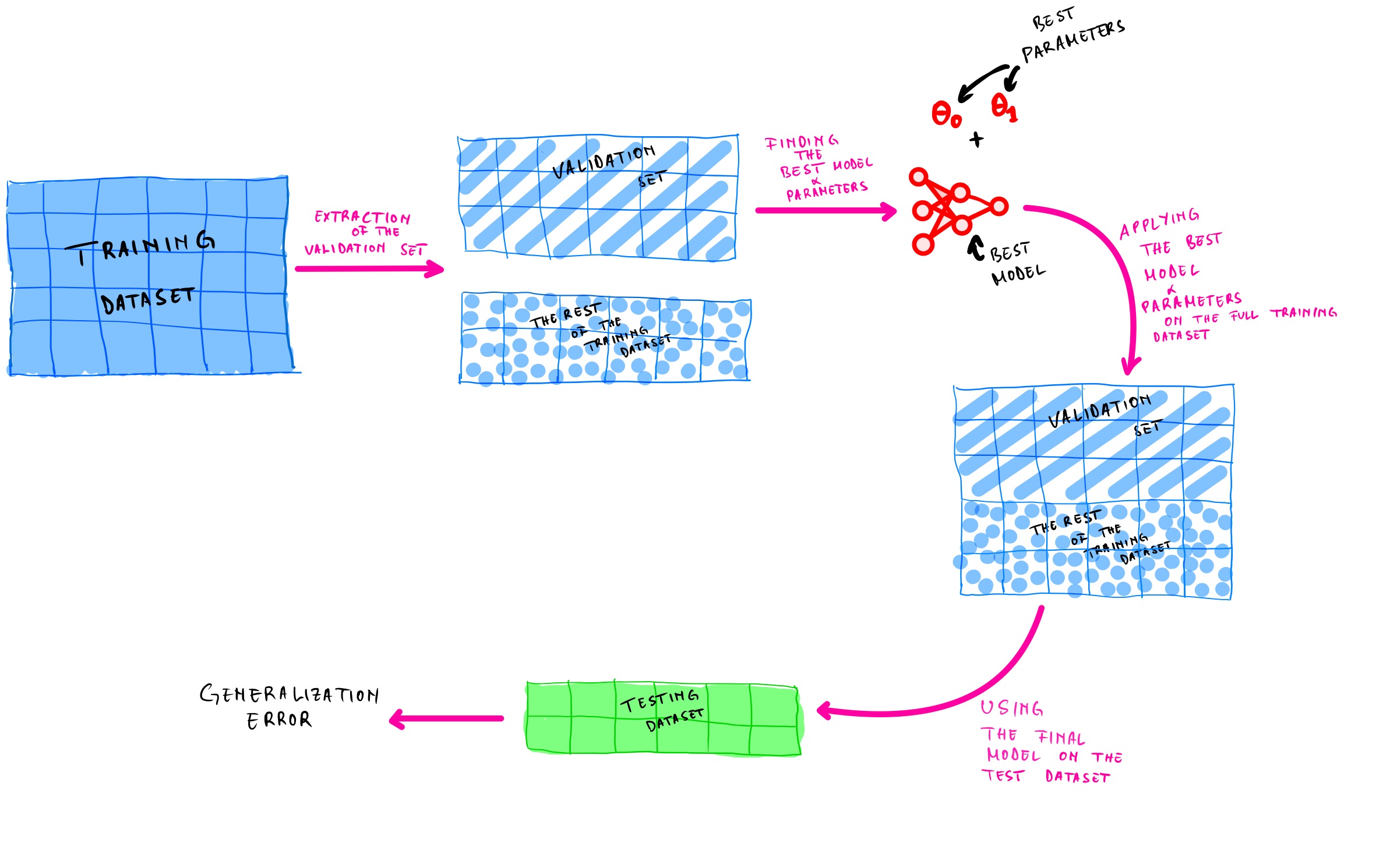
However, the main challenge here will be to know how big (or small) is the validation set compare to the training set. Why would this be a challenge, may you ask?

Because we will train the final model on the whole training dataset, so we must avoid as much as possible selecting a model that is not representative of the entire training set. So how can we overcome this?

We can use cross-validation to divide the training set into small validation sets called k-fold blocks where k represents the number of small validation sets. For example, if we divide the training set into ten smaller validation sets, we will have ten-fold cross-validation. Each model is tested on one small validation set after being trained on the other sets (for the previously mentioned ten-fold cross-validation, the model will be tested on one set and trained on the remaining nine sets). The only disadvantage of using cross-validation is that it requires a lot of computing power because the training time is multiply by the number of validation sets k.

6. Conclusion

Wow! You have to have made it until the end! Congratulation! You have learned a lot about machine learning in this post. It is okay to go through this post twice or thrice to grasp everything. But don’t worry! You will strengthen your understanding more when we start doing end-to-end machine learning projects. We will practice most of the theoretical concepts that we have discussed in this post in future posts.

Finally, here is a recap of the main points we have discovered in this post:

• Machine learning is the computer’s ability to learn through data and make predictions on new data without being explicitly hardcoded.

• If the problem you are trying to solve requires a lot of fine-tuning, or is complex, or requires a large amount of data, only then use machine learning

• There are different types of machine learning systems grouped b, first how they train (supervised, unsupervised, semisupervised or reinforcement learning). Second, how they learn (batch or online learning). Third, how they generalize (instance-based or model-based learning).

  Most machine learning projects follow this blueprint:

  Gather data -> clean data -> Split the dataset into training and testing data -> feed the training dataset -> test using the testing dataset -> find the generalization error of the model -> improve the generalization error

• Machine learning faces some challenges caused by the data and the model

• To know the accuracy of a machine learning model, we have to test it to find the generalization error. If satisfied with it, we select the best model and its hyperparameters using the validation set and the cross-validation.

Note: Always try to first use traditional programming before using machine learning (or deep learning). Don’t be like this guy below :)

Image credit: cutting-sword-credit

In the next post, we will work on an end-to-end machine learning project. I hope you enjoyed this post as much as I did. Find the jupyter notebook version of this post on my GitHub profile here.

Thank you again for going through this tutorial with me. I hope you have learned one or two things. If you like this post, please subscribe to stay updated with new posts, and if you have a thought or a question, I would love to hear it by commenting below. Remember, practice makes perfect! Keep on learning!

Share this post on