Great to see you again here! In this last post of the Pandas series, we will continue exploring advanced DataFrame exercises. Pandas is easer to learn than NumPy, in my opinion. Its documentation is well written, so don’t be shy! Read its documentation throughout if you get stuck here.

Let’s get started by importing NumPy and Pandas.

import numpy as np
import pandas as pd 

Ex 51: How to get the row number of the nth largest value in a column?

Q: Find the row position of the 5th largest value of column a of the_dataframe.

from numpy.random import default_rng
np.random.seed(42)
rng = default_rng()
the_dataframe = pd.DataFrame(rng.choice(30, size=30, replace=False).reshape(10,-1), columns=list('abc'))

the_dataframe

	a	b	c
0	16	11	9
1	25	22	15
2	1	18	8
3	27	12	3
4	19	17	20
5	0	24	28
6	23	13	21
7	29	5	2
8	7	10	26
9	6	14	4

Note: We import and use default_rng to generated no duplicate values in the DataFrame and use random.seed to always generate the same numbers even on a different computer.

Desired out

# The row with the 5th largest number is 6

1st Method

row_fifth_largest_num = the_dataframe["a"].sort_values(reversed)[::-1].index[4]

print("The row with the 5th largest number is {}".format(row_fifth_largest_num))

The row with the 5th largest number is 6

We first sort the values in column a, and then reverse it. To get the index(the row number) of the 5th position, we pass in 4 in the index (indexes start from 0).

2nd Method

row_fifth_largest_num = the_dataframe["a"].argsort()[::-1][5]

print("The row with the 5th largest number is {}".format(row_fifth_largest_num))

The row with the 5th largest number is 6

Another way is by using argsort which will return sorted indexes according to the values in those indexes. Then we reverse those indexes using [::1] and get the fifth element using [5].

Ex 52: How to find the position of the nth largest value greater than a given value?

Q: In the_serie find the position of the 2nd largest value greater than the mean.

np.random.seed(42)
the_serie = pd.Series(np.random.randint(1, 100, 15))

the_serie

0     52
1     93
2     15
3     72
4     61
5     21
6     83
7     87
8     75
9     75
10    88
11    24
12     3
13    22
14    53
dtype: int64

Desired output

# The mean is 55.0 and the row of the second largest number is 3

Solution

the_mean = np.mean(the_serie.values).round()

the_mean

55.0

greater_than_mean_arr = the_serie.where(the_serie > the_mean).dropna().sort_values()

row_second_largest_num = greater_than_mean_arr.index[1]

row_second_largest_num

3

print("The mean is {} and the row of the second largest number is {}".format(the_mean, row_second_largest_num))

The mean is 55.0 and the row of the second largest number is 3

We start by calculating the mean of the values in the series using np.mean and round it. Then we use where to get all rows with the values superior to the mean.

We drop NaN values (which are values inferior to the mean) and sort the remaining values to finally get the second value in the sorted series using .index[1] which correspond to the second largest number superior to the mean.

Ex 53: How to get the last n rows of a DataFrame with row sum > 100?

Q: Get the last two rows of the_dataframe whose row sum is superior to 100.

np.random.seed(42)
the_dataframe = pd.DataFrame(np.random.randint(10, 40, 60).reshape(-1, 4))

the_dataframe

	0	1	2	3
0	16	29	38	24
1	20	17	38	30
2	16	35	28	32
3	20	20	33	30
4	13	17	33	12
5	31	30	11	33
6	21	39	15	11
7	37	30	10	21
8	35	31	38	21
9	34	26	36	36
10	19	37	37	25
11	24	39	39	24
12	39	28	21	32
13	29	34	12	14
14	28	16	30	18

Desired output

Solution

rows_sum = the_dataframe.sum(axis=1).sort_values()

rows_sum

4      75
6      86
13     89
14     92
7      98
3     103
1     105
5     105
0     107
2     111
10    118
12    120
8     125
11    126
9     132
dtype: int64

rows_sum_greater_100 = rows_sum.where(rows_sum > 100).dropna()
rows_sum_greater_100

3     103.0
1     105.0
5     105.0
0     107.0
2     111.0
10    118.0
12    120.0
8     125.0
11    126.0
9     132.0
dtype: float64

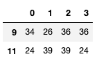
the_dataframe.iloc[rows_sum_greater_100[::-1][:2].index]

	0	1	2	3
9	34	26	36	36
11	24	39	39	24

We calculate a series with of the sum of all the elements row-wise and sort it. We then use where function to get only the row with element greater than 100 and drop the rest using dropna function.

Finally, we reverse that row using [::-1] and get the indexes first two rows using indexing from 0 to 2 (exclusive). We replace those indexes in the original dataframe to get the two rows using iloc.

Ex 54: How to find and cap outliers from a series or DataFrame column?

Q: Replace all values of the_serie lower to the 5th percentile and greater than 95th percentile respectively with the 5th and 95th percentile value.

the_serie = ser = pd.Series(np.logspace(-2, 2, 30))

Desired output

# 0      0.016049
# 1      0.016049
# 2      0.018874
# 3      0.025929
# 4      0.035622
# 5      0.048939
# 6      0.067234
# 7      0.092367
# 8      0.126896
# 9      0.174333
# 10     0.239503
# 11     0.329034
# 12     0.452035
# 13     0.621017
# 14     0.853168
# 15     1.172102
# 16     1.610262
# 17     2.212216
# 18     3.039195
# 19     4.175319
# 20     5.736153
# 21     7.880463
# 22    10.826367
# 23    14.873521
# 24    20.433597
# 25    28.072162
# 26    38.566204
# 27    52.983169
# 28    63.876672
# 29    63.876672
# dtype: float64

Solution

low_perc = the_serie.quantile(q=0.05)
low_perc

0.016049294076965887

high_perc = the_serie.quantile(q=0.95)
high_perc

63.876672220183934

the_serie.where(the_serie > low_perc, other=low_perc, inplace=True) 

the_serie.where(the_serie < high_perc, other=high_perc, inplace=True) 

the_serie

0      0.016049
1      0.016049
2      0.018874
3      0.025929
4      0.035622
5      0.048939
6      0.067234
7      0.092367
8      0.126896
9      0.174333
10     0.239503
11     0.329034
12     0.452035
13     0.621017
14     0.853168
15     1.172102
16     1.610262
17     2.212216
18     3.039195
19     4.175319
20     5.736153
21     7.880463
22    10.826367
23    14.873521
24    20.433597
25    28.072162
26    38.566204
27    52.983169
28    63.876672
29    63.876672
dtype: float64

We first calculate the 5th and the 95th percentile using the quantile function and pass in q the number 0.05 and 0.95 respectively. Then we call the where function on the original series, pass in the condition as the_serie > low_perc.

This condition will target the elements superior to the 5th percentile and set other which is the remaining element (inferior to the 5th percentile) to be the 5th percentile. The assignment will replace all the values in the series lower than the 5th percentile by the 5th percentile value. Finally, we set inplace to True.

We do the same for the 95th percentile, just that this time we are targeting elements inferior to the 95th percentile and set other to the value of the 95th percentile.

Ex 55: How to reshape a DataFrame to the largest possible square after removing the negative values?

Q: Reshape the_dataframe to the largest possible square with negative values removed. Drop the smallest values if need be. The order of the positive numbers in the result should remain the same as the original.

np.random.seed(42)
the_dataframe = pd.DataFrame(np.random.randint(-20, 50, 100).reshape(10,-1))
the_dataframe

	0	1	2	3	4	5	6	7	8	9
0	31	-6	40	0	3	-18	1	32	-19	9
1	17	-19	43	39	0	12	37	1	28	38
2	21	39	-6	41	41	26	41	30	34	43
3	-18	30	-14	0	18	-3	-17	39	-7	-12
4	32	-19	39	23	-13	26	14	15	29	-17
5	-19	-15	33	-17	33	42	-3	23	13	41
6	-7	27	-6	41	19	32	3	5	39	20
7	8	-6	24	44	-12	-20	-13	42	-10	-13
8	14	14	12	-16	20	7	-14	-9	13	12
9	27	2	41	16	23	14	44	26	-18	-20

Desired output

# array([[31., 40.,  3., 32.,  9., 17., 43., 39.],
#        [12., 37., 28., 38., 21., 39., 41., 41.],
#        [26., 41., 30., 34., 43., 30., 18., 39.],
#        [32., 39., 23., 26., 14., 15., 29., 33.],
#        [33., 42., 23., 13., 41., 27., 41., 19.],
#        [32.,  3.,  5., 39., 20.,  8., 24., 44.],
#        [42., 14., 14., 12., 20.,  7., 13., 12.],
#        [27.,  2., 41., 16., 23., 14., 44., 26.]])

Solution

Step 1: Remove the negatives

the_arr = the_dataframe[the_dataframe > 0].values.flatten()
the_arr

array([31., nan, 40., nan,  3., nan,  1., 32., nan,  9., 17., nan, 43.,
       39., nan, 12., 37.,  1., 28., 38., 21., 39., nan, 41., 41., 26.,
       41., 30., 34., 43., nan, 30., nan, nan, 18., nan, nan, 39., nan,
       nan, 32., nan, 39., 23., nan, 26., 14., 15., 29., nan, nan, nan,
       33., nan, 33., 42., nan, 23., 13., 41., nan, 27., nan, 41., 19.,
       32.,  3.,  5., 39., 20.,  8., nan, 24., 44., nan, nan, nan, 42.,
       nan, nan, 14., 14., 12., nan, 20.,  7., nan, nan, 13., 12., 27.,
        2., 41., 16., 23., 14., 44., 26., nan, nan])

We use indexing with [] to get all the positive elements in the_dataframe and reshaped them into a 1D array using flatten() function to finally store it into the_arr.

pos_arr = the_arr[~np.isnan(the_arr)]

np.isnan(the_arr)

array([False,  True, False,  True, False,  True, False, False,  True,
       False, False,  True, False, False,  True, False, False, False,
       False, False, False, False,  True, False, False, False, False,
       False, False, False,  True, False,  True,  True, False,  True,
        True, False,  True,  True, False,  True, False, False,  True,
       False, False, False, False,  True,  True,  True, False,  True,
       False, False,  True, False, False, False,  True, False,  True,
       False, False, False, False, False, False, False, False,  True,
       False, False,  True,  True,  True, False,  True,  True, False,
       False, False,  True, False, False,  True,  True, False, False,
       False, False, False, False, False, False, False, False,  True,
        True])

pos_arr

array([31., 40.,  3.,  1., 32.,  9., 17., 43., 39., 12., 37.,  1., 28.,
       38., 21., 39., 41., 41., 26., 41., 30., 34., 43., 30., 18., 39.,
       32., 39., 23., 26., 14., 15., 29., 33., 33., 42., 23., 13., 41.,
       27., 41., 19., 32.,  3.,  5., 39., 20.,  8., 24., 44., 42., 14.,
       14., 12., 20.,  7., 13., 12., 27.,  2., 41., 16., 23., 14., 44.,
       26.])

To drop the nan in the array, we use indexing and isnan function to return a boolean array where False represent a non nan value and True is a position of a nan value. We then ~ sign to inverse the boolean to get True in where there is non nan value. Now we get a new array with no nan values.

Step 2: Find side-length of largest possible square

len(pos_arr)

66

n = int(np.floor(np.sqrt(pos_arr.shape[0])))

n

8

To search for the largest possible square, we get first the length of the array using shape function (we could also use len() function). We then find the square root of the number of elements in the array and remove the decimal using floor function cast it to an integer.

Step 3: Take top n^2 items without changing positions

top_indexes = np.argsort(pos_arr)[::-1]

top_indexes

array([64, 49, 22,  7, 50, 35, 16, 40, 19, 17, 60, 38,  1, 15, 27,  8, 25,
       45, 13, 10, 21, 33, 34, 42, 26,  4,  0, 23, 20, 32, 12, 39, 58, 65,
       29, 18, 48, 62, 36, 28, 14, 54, 46, 41, 24,  6, 61, 31, 63, 51, 52,
       30, 37, 56,  9, 57, 53,  5, 47, 55, 44, 43,  2, 59, 11,  3])

np.take(pos_arr, sorted(top_indexes[:n**2])).reshape(n,-1)

array([[31., 40.,  3., 32.,  9., 17., 43., 39.],
       [12., 37., 28., 38., 21., 39., 41., 41.],
       [26., 41., 30., 34., 43., 30., 18., 39.],
       [32., 39., 23., 26., 14., 15., 29., 33.],
       [33., 42., 23., 13., 41., 27., 41., 19.],
       [32.,  3.,  5., 39., 20.,  8., 24., 44.],
       [42., 14., 14., 12., 20.,  7., 13., 12.],
       [27.,  2., 41., 16., 23., 14., 44., 26.]])

We then sort the element indexes using argsort and reverse the order into a descending order using slicing [::-1] and store it in top_indexes.

Finally, we use take NumPy function that takes the pos_arr and as indices the sorted top_indexes (from the first indices up to n raised to the power of 2). Then we reshape the array using (n,-1) to let Pandas figure out the best reshape argument to use depending on n value.

Ex 56: How to swap two rows of a DataFrame?

Q: Swap rows 1 and 2 in the_dataframe

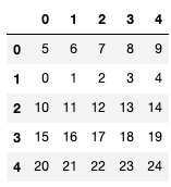
the_dataframe = pd.DataFrame(np.arange(25).reshape(5, -1))

the_dataframe

	0	1	2	3	4
0	0	1	2	3	4
1	5	6	7	8	9
2	10	11	12	13	14
3	15	16	17	18	19
4	20	21	22	23	24

Desired solution

Solution

def row_swap(the_dataframe,row_index_1,row_index_2):
    row_1, row_2 = the_dataframe.iloc[row_index_1,:].copy(), the_dataframe.iloc[row_index_2,:].copy()
    the_dataframe.iloc[row_index_1,:], the_dataframe.iloc[row_index_2,:] = row_2, row_1
    return the_dataframe

row_swap(the_dataframe,0,1)

	0	1	2	3	4
0	5	6	7	8	9
1	0	1	2	3	4
2	10	11	12	13	14
3	15	16	17	18	19
4	20	21	22	23	24

We create a function that performs the swap it takes in the dataframe and the two indexes of the rows that need to be swap. We then copy the rows using iloc and store them in row_1 and row_2.

To do the swap, we do the opposite of what we did by assigning row_1 and row_2 to the equivalent row index we want to change to occur. So row_2 will be assigned to row_index_1 and row_1 will be assigned to row_index_2. Finally, we return the_dataframe.

Ex 57: How to reverse the rows of a DataFrame?

Q: Reverse all the rows of a DataFrame.

the_dataframe = pd.DataFrame(np.arange(25).reshape(5, -1))

the_dataframe

	0	1	2	3	4
0	0	1	2	3	4
1	5	6	7	8	9
2	10	11	12	13	14
3	15	16	17	18	19
4	20	21	22	23	24

Desired output

Solution

1st method

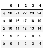
the_dataframe.iloc[::-1]

	0	1	2	3	4
4	20	21	22	23	24
3	15	16	17	18	19
2	10	11	12	13	14
1	5	6	7	8	9
0	0	1	2	3	4

2nd method

the_dataframe[::-1]

	0	1	2	3	4
4	20	21	22	23	24
3	15	16	17	18	19
2	10	11	12	13	14
1	5	6	7	8	9
0	0	1	2	3	4

To reverse the dataframe row-wise, we use indexing with [::-1]. The second method is the short form of the first method we used iloc.

Note: In Exercise 75, we will see how to achieve the same result column-wise.

Ex 58: How to create one-hot encodings of a categorical variable (dummy variables)?

Q: Get one-hot encodings for column a in the dataframe the_dataframe and append it as columns.

the_dataframe = pd.DataFrame(np.arange(25).reshape(5,-1), columns=list('abcde'))
the_dataframe

	a	b	c	d	e
0	0	1	2	3	4
1	5	6	7	8	9
2	10	11	12	13	14
3	15	16	17	18	19
4	20	21	22	23	24

Desired output

Solution

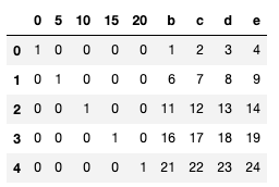
one_hot = pd.get_dummies(the_dataframe["a"])

one_hot

	0	5	10	15	20
0	1	0	0	0	0
1	0	1	0	0	0
2	0	0	1	0	0
3	0	0	0	1	0
4	0	0	0	0	1

pd.concat([one_hot, the_dataframe[["b","c","d","e"]]],axis=1)

	0	5	10	15	20	b	c	d	e
0	1	0	0	0	0	1	2	3	4
1	0	1	0	0	0	6	7	8	9
2	0	0	1	0	0	11	12	13	14
3	0	0	0	1	0	16	17	18	19
4	0	0	0	0	1	21	22	23	24

We get the one-hot encoding of column a by using the get_dummies function and pass in the column a.

To append the newly created one_hot, we use concat and pass in one_hot and the remaining columns of dataframe (except column a). Finally, we set the axis to 1 since we want to concatenate column-wise.

Ex 59: Which column contains the highest number of row-wise maximum values?

Q: Obtain the column name with the highest number of row-wise in the_dataframe.

np.random.seed(42)
the_dataframe = pd.DataFrame(np.random.randint(1,100, 40).reshape(10, -1))

Desired output

# The column name with the highest number of row-wise is 0

Solution

row_high_num = the_dataframe.sum(axis=0).argmax()

print("The column name with the highest number of row-wise is {}".format(row_high_num))

The column name with the highest number of row-wise is 0

To get the row with the largest sum row-wise, we use the sum function and pass in the axis argument set to 0 (telling Pandas to calculate the sum of elements row-wise) and then use argmax to get the index with the highest value in the series.

Ex 60: How to know the maximum possible correlation value of each column against other columns?

Q: Compute the maximum possible absolute correlation value of each column against other columns in the_dataframe.

np.random.seed(42)
the_dataframe = pd.DataFrame(np.random.randint(1,100, 80).reshape(8, -1), columns=list('pqrstuvwxy'), index=list('abcdefgh'))

Desired output

# array([0.81941445, 0.84466639, 0.44944264, 0.44872809, 0.81941445,
#        0.80618428, 0.44944264, 0.5434561 , 0.84466639, 0.80618428])

Solution

abs_corr = np.abs(the_dataframe.corr())

abs_corr

	p	q	r	s	t	u	v	w	x	y
p	1.000000	0.019359	0.088207	0.087366	0.819414	0.736955	0.070727	0.338139	0.163112	0.665627
q	0.019359	1.000000	0.280799	0.121217	0.172215	0.262234	0.304781	0.042748	0.844666	0.243317
r	0.088207	0.280799	1.000000	0.184988	0.223515	0.017763	0.449443	0.127091	0.228455	0.018350
s	0.087366	0.121217	0.184988	1.000000	0.210879	0.096695	0.422290	0.306141	0.100174	0.448728
t	0.819414	0.172215	0.223515	0.210879	1.000000	0.576720	0.334690	0.543456	0.047136	0.273478
u	0.736955	0.262234	0.017763	0.096695	0.576720	1.000000	0.137836	0.352145	0.363597	0.806184
v	0.070727	0.304781	0.449443	0.422290	0.334690	0.137836	1.000000	0.158152	0.188482	0.033227
w	0.338139	0.042748	0.127091	0.306141	0.543456	0.352145	0.158152	1.000000	0.325939	0.071704
x	0.163112	0.844666	0.228455	0.100174	0.047136	0.363597	0.188482	0.325939	1.000000	0.338705
y	0.665627	0.243317	0.018350	0.448728	0.273478	0.806184	0.033227	0.071704	0.338705	1.000000

max_abs_corr = abs_corr.apply(lambda x: sorted(x)[-2]).values

max_abs_corr

array([0.81941445, 0.84466639, 0.44944264, 0.44872809, 0.81941445,
       0.80618428, 0.44944264, 0.5434561 , 0.84466639, 0.80618428])

We first calculate the absolute correlation the whole dataset. We use the corr() function and pass it as the argument to the NumPy function abs to get the absolute values (non-negative values).

Now that we have the absolute correction, use lambda expression with the apply function to find the highest correlation value in each row.

We sorted first each row (represented by x in the lambda expression), secondly get the second last element in the row using indexing. The reason why we get the second-highest value instead of the last one is because the last value is 1 (calculated from the correlation of the same column). We then form an array with the highest correlation values in each row.

Ex 61: How to create a column containing the minimum by the maximum of each row?

Q: Compute the minimum-by-maximum for every row of the_dataframe.

np.random.seed(42)
the_dataframe = pd.DataFrame(np.random.randint(1,100, 80).reshape(8, -1))
the_dataframe

	0	1	2	3	4	5	6	7	8	9
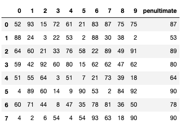
0	52	93	15	72	61	21	83	87	75	75
1	88	24	3	22	53	2	88	30	38	2
2	64	60	21	33	76	58	22	89	49	91
3	59	42	92	60	80	15	62	62	47	62
4	51	55	64	3	51	7	21	73	39	18
5	4	89	60	14	9	90	53	2	84	92
6	60	71	44	8	47	35	78	81	36	50
7	4	2	6	54	4	54	93	63	18	90

Desired output

# 0    0.161290
# 1    0.022727
# 2    0.230769
# 3    0.163043
# 4    0.041096
# 5    0.021739
# 6    0.098765
# 7    0.021505
# dtype: float64

Solution

1st Method

the_min = the_dataframe.min(axis=1)

the_max = the_dataframe.max(axis=1)

min_by_max = the_min/the_max

min_by_max

0    0.161290
1    0.022727
2    0.230769
3    0.163043
4    0.041096
5    0.021739
6    0.098765
7    0.021505
dtype: float64

The easiest way to solve this problem is to find the minimum values in each column using the min function by setting the axis to 1. We do the same for the maximum to finally divide the minimum values by the maximum values.

2nd Method

the_dataframe.apply(lambda x: np.min(x)/np.max(x), axis=1)

0    0.161290
1    0.022727
2    0.230769
3    0.163043
4    0.041096
5    0.021739
6    0.098765
7    0.021505
dtype: float64

The previous method uses three lines of codes we can write in one line of code. We use the lambda expression to calculate the division of the minimum by the maximum of x and set axis to 1.

Ex 62: How to create a column that contains the penultimate value in each row?

Q: Create a new column penultimate which has the second-largest value of each row of the_dataframe.

np.random.seed(42)
the_dataframe = pd.DataFrame(np.random.randint(1,100, 80).reshape(8, -1))

Desire output

Solution

the_dataframe['penultimate'] = the_dataframe.apply(lambda x: x.sort_values().unique()[-2], axis=1)

As previously seen, to solve this type of challenge, we use a lambda expression with the apply function. We first set axis to 1 as we are calculating the values row-wise and in the lambda expression, we sort x ignore the duplicate with ignore function and return the second largest value using indexing [-2].

Ex 63: How to normalize all columns in a dataframe?

Q1: Normalize all columns of the_dataframe by subtracting the column mean and divide by standard deviation.

Q2: Range all columns values of the_dataframe such that the minimum value in each column is 0 and max is 1.

Note: Don’t use external packages like sklearn.

np.random.seed(42)
the_dataframe = pd.DataFrame(np.random.randint(1,100, 80).reshape(8, -1))

Desired output

Q1

Q2

Solution

Q1

the_dataframe.apply(lambda x: (x - x.mean()) / x.std(),axis=0)

	0	1	2	3	4	5	6	7	8	9
0	0.144954	1.233620	-0.722109	1.495848	0.478557	-0.471883	0.718777	0.860589	1.241169	0.434515
1	1.372799	-0.977283	-1.096825	-0.434278	0.192317	-1.101061	0.894088	-1.017060	-0.475588	-1.680126
2	0.554235	0.176231	-0.534751	-0.009651	1.015256	0.753357	-1.420023	0.926472	0.034799	0.897999
3	0.383701	-0.400526	1.682318	1.032617	1.158376	-0.670571	-0.017531	0.037059	-0.057999	0.057935
4	0.110847	0.016021	0.807981	-1.167726	0.120757	-0.935488	-1.455085	0.399412	-0.429189	-1.216643
5	-1.492172	1.105451	0.683076	-0.743098	-1.382001	1.813025	-0.333092	-1.939414	1.658759	0.926966
6	0.417808	0.528694	0.183455	-0.974714	-0.022362	-0.008279	0.543466	0.662942	-0.568386	-0.289677
7	-1.492172	-1.682209	-1.003146	0.801002	-1.560900	0.620899	1.069400	0.070000	-1.403565	0.869031

To solve this issue, we need to know the formula for normalizing. The formulation is as follow:

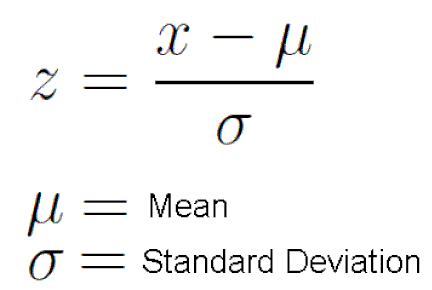
So now we can proceed with the apply function and lambda expression. We set the axis to 0 since we are normalizing column-wise and with the lambda expression we do the calculation according to the formula above.

Q2

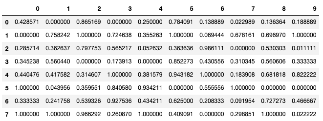
the_dataframe.apply(lambda x: (x.max() - x)/(x.max()-x.min()),axis=0)

	0	1	2	3	4	5	6	7	8	9
0	0.428571	0.000000	0.865169	0.000000	0.250000	0.784091	0.138889	0.022989	0.136364	0.188889
1	0.000000	0.758242	1.000000	0.724638	0.355263	1.000000	0.069444	0.678161	0.696970	1.000000
2	0.285714	0.362637	0.797753	0.565217	0.052632	0.363636	0.986111	0.000000	0.530303	0.011111
3	0.345238	0.560440	0.000000	0.173913	0.000000	0.852273	0.430556	0.310345	0.560606	0.333333
4	0.440476	0.417582	0.314607	1.000000	0.381579	0.943182	1.000000	0.183908	0.681818	0.822222
5	1.000000	0.043956	0.359551	0.840580	0.934211	0.000000	0.555556	1.000000	0.000000	0.000000
6	0.333333	0.241758	0.539326	0.927536	0.434211	0.625000	0.208333	0.091954	0.727273	0.466667
7	1.000000	1.000000	0.966292	0.260870	1.000000	0.409091	0.000000	0.298851	1.000000	0.022222

To change the values in the dataframe to put them on a scale of 0 to 1 we use the following formulaMAX - Z / MAX - MIN and do the same as we did in Q1.

Ex 64: How to compute the correlation of each row with the succeeding row?

Q: Compute the correlation of each row with its previous row, round the result by 2.

np.random.seed(42)
the_dataframe = pd.DataFrame(np.random.randint(1,100, 80).reshape(8, -1))

Desired output

# [0.31, -0.14, -0.15, 0.47, -0.32, -0.07, 0.12]

Solution

[the_dataframe.iloc[i].corr(the_dataframe.iloc[i+1]).round(2) for i in range(the_dataframe.shape[0]-1)]

[0.31, -0.14, -0.15, 0.47, -0.32, -0.07, 0.12]

We first loop through the range of the number of rows in the dataframe using shape function (excluding the last row because we are comparing a pair of rows). We then call the corr function on each row using the iloc function and pass in the corr function the next row location by adding 1 to i. Finally, we round the result by two decimal point and place it in a list comprehension.

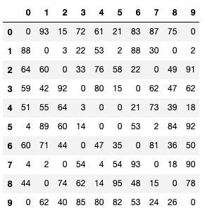
Ex 65: How to replace both the diagonals of dataframe with 0?

Q: Replace both values in both diagonals of the_dataframe with 0.

np.random.seed(42)
the_dataframe = pd.DataFrame(np.random.randint(1,100, 100).reshape(10, -1))

Desired output

Solution

for i in range(the_dataframe.shape[0]):
    the_dataframe.iat[i,i] = 0
    the_dataframe.iat[the_dataframe.shape[0]-i-1,i] = 0

the_dataframe

	0	1	2	3	4	5	6	7	8	9
0	0	93	15	72	61	21	83	87	75	0
1	88	0	3	22	53	2	88	30	0	2
2	64	60	0	33	76	58	22	0	49	91
3	59	42	92	0	80	15	0	62	47	62
4	51	55	64	3	0	0	21	73	39	18
5	4	89	60	14	0	0	53	2	84	92
6	60	71	44	0	47	35	0	81	36	50
7	4	2	0	54	4	54	93	0	18	90
8	44	0	74	62	14	95	48	15	0	78
9	0	62	40	85	80	82	53	24	26	0

We are going to fill both diagonal (right-to-left and left-to-right) with 0. There is a NumPy function called fill_diagnol to replace values on the left-to-right diagonal but the issue with this function is that it does not replace the right-to-left diagonal as well. We can’t use this function, therefore.

To solve this challenge, we first loop through rows in the dataframe and then for each loop we are to replace two elements at a specific position with 0 row-wise. For the left-to-right diagonal, we use the iat function which takes in at the first position index the row number and at the second position the column number, we use i for both positions. For the right-to-left diagonal, we use the iat function again but this time the first position we calculate the total number rows in the dataframe minus i (as i changes because of the loop) minus 1 because indexes start from 0 and for the second position corresponding to the columns we use i.

Ex 66: How to get the particular group of a groupby dataframe by key?

Q: This is a question related to the understanding of grouped dataframe. From df_grouped, get the group belonging to apple as a dataframe.

np.random.seed(42)
the_dataframe = pd.DataFrame({'col1': ['apple', 'banana', 'orange'] * 3,
                   'col2': np.random.rand(9),
                   'col3': np.random.randint(0, 15, 9)})

df_grouped = the_dataframe.groupby(['col1'])

the_dataframe

	col1	col2	col3
0	apple	0.374540	7
1	banana	0.950714	2
2	orange	0.731994	5
3	apple	0.598658	4
4	banana	0.156019	1
5	orange	0.155995	7
6	apple	0.058084	11
7	banana	0.866176	13
8	orange	0.601115	5

df_grouped

<pandas.core.groupby.generic.DataFrameGroupBy object at 0x7fd121fc30d0>

Desired output

#     col1      col2  col3
# 0  apple  0.374540     7
# 3  apple  0.598658     4
# 6  apple  0.058084    11

Solution

1st Method

df_grouped.get_group("apple")

	col1	col2	col3
0	apple	0.374540	7
3	apple	0.598658	4
6	apple	0.058084	11

To get the group belonging to apple we call get_group on the df_grouped.

2nd Method

for i, grp_val in df_grouped:
    if i == "apple":
        print(grp_val)

    col1      col2  col3
0  apple  0.374540     7
3  apple  0.598658     4
6  apple  0.058084    11

Alternatively, we loop through all the elements in df_grouped and use the if statement to print the columns in the apple group.

Ex 67: How to get the nth largest value of a column when grouped by another column?

Q: In the_dataframe, find the second largest value of taste for banana.

np.random.seed(42)
the_dataframe = pd.DataFrame({'fruit': ['apple', 'banana', 'orange'] * 3,
                   'taste': np.random.rand(9),
                   'price': np.random.randint(0, 15, 9)})

Desired output

# 0.8661761457749352

Solution

the_dataframe

	fruit	taste	price
0	apple	0.374540	7
1	banana	0.950714	2
2	orange	0.731994	5
3	apple	0.598658	4
4	banana	0.156019	1
5	orange	0.155995	7
6	apple	0.058084	11
7	banana	0.866176	13
8	orange	0.601115	5

df_grouped = the_dataframe.groupby(by="fruit")

sorted(df_grouped.get_group("banana")["taste"])[-2]

0.8661761457749352

Just like we did in the previous exercise, we first group the dataframe using the values in the fruit column and store it in df_grouped. Then we get taste column for banana using get_group function and sort it out. Finally, to get the second largest element, we use indexing [-2].

Ex 68: How to compute grouped mean on pandas DataFrame and keep the grouped column as another column (not index)?

Q: In the_dataframe, Compute the mean price of every fruit, while keeping the fruit as another column instead of an index.

np.random.seed(42)
the_dataframe = pd.DataFrame({'fruit': ['apple', 'banana', 'orange'] * 3,
                   'taste': np.random.rand(9),
                   'price': np.random.randint(0, 15, 9)})

Desired output

Solution

1st Method

the_dataframe.groupby(by="fruit").mean()["price"].reset_index()

	fruit	price
0	apple	7.333333
1	banana	5.333333
2	orange	5.666667

The most straightforward way to go about this exercise is to group the dataframe by fruit and get the mean of the numerical columns grouped by price and reset the index using reset_index which will change the index from fruit column to regular ascending numerical index.

2nd Method

the_dataframe.groupby(by="fruit",as_index=False)["price"].mean()

	fruit	price
0	apple	7.333333
1	banana	5.333333
2	orange	5.666667

Alternatively, we can reset the index using the as_index parameter from the groupby function.

Ex 69: How to join two DataFrames by 2 columns so that they have only the common rows?

Q: Join dataframes the_dataframe_1 and the_dataframe_2 by fruit-pazham and weight-kilo.

the_dataframe_1 = pd.DataFrame({'fruit': ['apple', 'banana', 'orange'] * 3,
                    'weight': ['high', 'medium', 'low'] * 3,
                    'price': np.random.randint(0, 15, 9)})

the_dataframe_2 = pd.DataFrame({'pazham': ['apple', 'orange', 'pine'] * 2,
                    'kilo': ['high', 'low'] * 3,
                    'price': np.random.randint(0, 15, 6)})

Desire output

Solution

the_dataframe_1

	fruit	weight	price
0	apple	high	1
1	banana	medium	11
2	orange	low	4
3	apple	high	0
4	banana	medium	11
5	orange	low	9
6	apple	high	5
7	banana	medium	12
8	orange	low	11

the_dataframe_2

	pazham	kilo	price
0	apple	high	8
1	orange	low	0
2	pine	high	10
3	apple	low	10
4	orange	high	14
5	pine	low	9

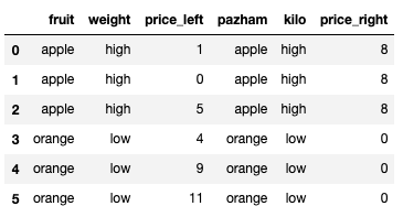
pd.merge(the_dataframe_1, the_dataframe_2, how="inner", left_on=["fruit","weight"], right_on=["pazham","kilo"], suffixes=["_left","_right"])

	fruit	weight	price_left	pazham	kilo	price_right
0	apple	high	1	apple	high	8
1	apple	high	0	apple	high	8
2	apple	high	5	apple	high	8
3	orange	low	4	orange	low	0
4	orange	low	9	orange	low	0
5	orange	low	11	orange	low	0

We use the merge to combine the two dataframes, and set how parameter to inner which means that we are only interested in rows with the same value in fruit and weight column on the left and pazham and kilo column on the right. Finally, we add suffix “_left” and “_right” on those columns.

Ex 70: How to remove rows from a DataFrame that are present in another DataFrame?

Q: From the_dataframe_1, remove the rows present in the_dataframe_2. All three columns values must be the same for the row to be drop.

np.random.seed(42)
the_dataframe_1 = pd.DataFrame({'fruit': ['apple', 'banana', 'orange'] * 3,
                    'weight': ['high', 'medium', 'low'] * 3,
                    'price': np.random.randint(0, 15, 9)})

the_dataframe_2 = pd.DataFrame({'pazham': ['apple', 'orange', 'pine'] * 2,
                    'kilo': ['high', 'low'] * 3,
                    'price': np.random.randint(0, 15, 6)})

Desired output

Solution

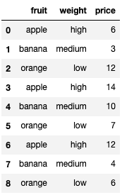
the_dataframe_1

	fruit	weight	price
0	apple	high	6
1	banana	medium	3
2	orange	low	12
3	apple	high	14
4	banana	medium	10
5	orange	low	7
6	apple	high	12
7	banana	medium	4
8	orange	low	6

the_dataframe_2

	pazham	kilo	price
0	apple	high	9
1	orange	low	2
2	pine	high	6
3	apple	low	10
4	orange	high	10
5	pine	low	7

the_dataframe_1[~the_dataframe_1.isin(the_dataframe_2).all(axis=1)]

	fruit	weight	price
0	apple	high	6
1	banana	medium	3
2	orange	low	12
3	apple	high	14
4	banana	medium	10
5	orange	low	7
6	apple	high	12
7	banana	medium	4
8	orange	low	6

We first get the element in the_dataframe_1 that are present in the_dataframe_2 using the isin function. A new dataframe with boolean values will is return where True represent a similar value between the_dataframe_1 and the_dataframe_2 and False represent a different value. We use all to get an AND operator function between the boolean values row-wise(axis set to 1). For example, in row 4, we’ll have “False” AND “False” AND “True” = “False”.

Finally, we use ~ to reverse all the boolean value (“False” becomes “True” and “True” becomes “False”) and use indexing into the_dataframe_1. We find out that we are keeping all the rows in the_dataframe_1 meaning that no row that is identical in the_dataframe_1 and the_dataframe_2.

Ex 71: How to get the positions where values of two columns match?

Q: Get the positions where values of two columns match

np.random.seed(42)
the_dataframe = pd.DataFrame({'fruit1': np.random.choice(['apple', 'orange', 'banana'], 10),
                    'fruit2': np.random.choice(['apple', 'orange', 'banana'], 10)})
the_dataframe

	fruit1	fruit2
0	banana	banana
1	apple	banana
2	banana	apple
3	banana	banana
4	apple	orange
5	apple	apple
6	banana	orange
7	orange	orange
8	banana	orange
9	banana	orange

Desired output

# [0, 3, 5, 7]

Solution

1st Method

the_dataframe.where(the_dataframe["fruit1"] == the_dataframe["fruit2"])

	fruit1	fruit2
0	banana	banana
1	NaN	NaN
2	NaN	NaN
3	banana	banana
4	NaN	NaN
5	apple	apple
6	NaN	NaN
7	orange	orange
8	NaN	NaN
9	NaN	NaN

list(the_dataframe.where(the_dataframe["fruit1"] == the_dataframe["fruit2"]).dropna().index)

[0, 3, 5, 7]

We first call the where function the the_dataframe with the condition that we need to the same fruit in column fruit1 and fruit2. We get boolean values dataframe with the rows where the values are the same and NaN where the values are different. We drop NaN using dropna function and extract the indexes. Finally, place the array into a list et voila!

2nd Method

list(np.where(the_dataframe["fruit1"] == the_dataframe["fruit2"])[0])

[0, 3, 5, 7]

Alternatevely w

list(np.where(the_dataframe["fruit1"] == the_dataframe["fruit2"])[0])

[0, 3, 5, 7]

np.where(the_dataframe["fruit1"] == the_dataframe["fruit2"])

(array([0, 3, 5, 7]),)

Alternatively, we can use the where function which returns a tuple with first element an array of the indexes where the condition is satisfied. We extract that array and cast it into a list. I prefer this second method as it is more concise.

Ex 72: How to create lags and leads of a column in a DataFrame?

Q: Create two new columns in the_dataframe, one of which is a lag1 (shift column a down by 1 row) of column a and the other is a lead1 (shift column b up by 1 row).

np.random.seed(42)
the_dataframe = pd.DataFrame(np.random.randint(1, 100, 20).reshape(-1, 4), columns = list('abcd'))

Desired output

Solution

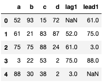
the_dataframe

	a	b	c	d
0	52	93	15	72
1	61	21	83	87
2	75	75	88	24
3	3	22	53	2
4	88	30	38	2

the_dataframe["lag1"] = the_dataframe["a"].shift(periods=1)
the_dataframe["lead1"] = the_dataframe["a"].shift(periods=-1)

the_dataframe

	a	b	c	d	lag1	lead1
0	52	93	15	72	NaN	61.0
1	61	21	83	87	52.0	75.0
2	75	75	88	24	61.0	3.0
3	3	22	53	2	75.0	88.0
4	88	30	38	2	3.0	NaN

To create a shift of values in a column upward or downward, we use the shift function on the desired column and pass in as the periods number 1 to shift upward or -1 to shift downward.

Ex 73: How to get the frequency of unique values in the entire DataFrame?

Q: Get the frequency of unique values in the entire DataFrame.

np.random.seed(42)
the_dataframe = pd.DataFrame(np.random.randint(1, 10, 20).reshape(-1, 4), columns = list('abcd'))

Desired output

# 8    5
# 5    4
# 7    3
# 6    2
# 4    2
# 3    2
# 2    2
# dtype: int64

Solution

the_dataframe

	a	b	c	d
0	7	4	8	5
1	7	3	7	8
2	5	4	8	8
3	3	6	5	2
4	8	6	2	5

pd.value_counts(the_dataframe.values.flatten())

8    5
5    4
7    3
6    2
4    2
3    2
2    2
dtype: int64

To get the frequency of unique values or how many time one value is repeated in the dataframe, we use value_counts and pass in the values of the_dataframe flattened which transform the dataframe from an n-dimensional dataframe into a 1D array.

Ex 74: How to split a text column into two separate columns?

Q: Split the string column in the_dataframe to form a dataframe with 3 columns as shown.

the_dataframe = pd.DataFrame(["Temperature, City    Province",
                              "33, Bujumbura    Bujumbura",
                              "30, Buganda    Cibitoke",
                              "25, Ncendajuru    Cankuzo",
                              "35, Giheta    Gitega"], 
                              columns=['row']
                            )

Desired output

Solution

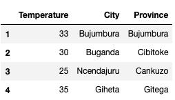
Step 1: split the string data

the_dataframe

	row
0	Temperature, City Province
1	33, Bujumbura Bujumbura
2	30, Buganda Cibitoke
3	25, Ncendajuru Cankuzo
4	35, Giheta Gitega

df_splitted = the_dataframe.row.str.split(pat=",|\t|    ", expand=True)

df_splitted

	0	1	2
0	Temperature	City	Province
1	33	Bujumbura	Bujumbura
2	30	Buganda	Cibitoke
3	25	Ncendajuru	Cankuzo
4	35	Giheta	Gitega

In this first step, we split the strings in the one column into three different columns. We call the split function on the str function from the row dataframe. We pass in as the pattern a regular expression that targets , or \t (tab) and (4 spaces) and set expand to True which expand the split strings into separate columns.

Step 2: Rename the columns

new_header = df_splitted.iloc[0]

new_header

0    Temperature
1           City
2       Province
Name: 0, dtype: object

df_splitted.columns = new_header

df_splitted

	Temperature	City	Province
0	Temperature	City	Province
1	33	Bujumbura	Bujumbura
2	30	Buganda	Cibitoke
3	25	Ncendajuru	Cankuzo
4	35	Giheta	Gitega

In step 2, we are going to use the first row strings as the column names. We first extract the row using iloc and store it in the new_header, Then assign it to columns of the dataframe.

Step 3: Drop the first row

df_splitted.drop(labels=0,axis="index",inplace=True)

df_splitted

	Temperature	City	Province
1	33	Bujumbura	Bujumbura
2	30	Buganda	Cibitoke
3	25	Ncendajuru	Cankuzo
4	35	Giheta	Gitega

Now that we have the column names all set, we no longer need that first row, so we are dropping it. We call the drop function on the dataframe and pass in as parameters label set to 0 to tell Pandas that we want to drop a row not a column, then set axis to index (We could also have used 0) to tell Pandas that we want to drop labels from the index. Finally set inplace to True to tell Pandas we don’t want a copy of the dataframe that instead, we want the change to occur in the original dataframe.

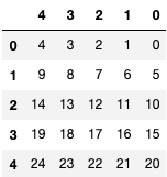
Ex 75: How to reverse the columns of a DataFrame?

Q: Reverse all the columns of a DataFrame.

np.random.seed(42)
the_dataframe = pd.DataFrame(np.arange(25).reshape(5, -1))

Desired output

Solution

the_dataframe[the_dataframe.columns[::-1]]

	4	3	2	1	0
0	4	3	2	1	0
1	9	8	7	6	5
2	14	13	12	11	10
3	19	18	17	16	15
4	24	23	22	21	20

This exercise is similar to exercise 57 the difference is that this time we are reversing columns instead of rows. To do the reversal, we first extract the columns and reverse them using indexing [::-1] and place it into the original dataframe using again indexing.

Conclusion

Yaaayy! We made it finally. In the last posts, we have explored more than 150 exercises on NumPy and Pandas. I am very confident that after going through all these exercises, you are ready to tackle the next step: Machine Learning with Scikit-learn. We will continue using NumPy in end-to-end Machine Learning projects coming in the next blog posts.

In the next post, we will introduce the common jargon used in Machine Learning, code our first Machine Learning algorithm and after that post we will start working on machine learning projects finally. I am super duper excited for the upcoming posts. Remember, practice makes perfect! Find the jupyter notebook version of this post on my GitHub profile here.

Thank you again for doing these exercises with me. I hope you have learned one or two things. If you like this post, please subscribe to stay updated with new posts, and if you have a thought or a question, I would love to hear it by commenting below. Cheers, and keep learning!

Share this post on